Diagnostic test performance: sensitivity, specificity, predictive values, likelihood ratios and ROC

Why this matters to the anaesthetist

Anaesthetic practice is saturated with diagnostic tests. Before induction you read a Mallampati score, a coagulation profile, an echocardiogram or a coronary CT; intraoperatively you act on a capnography trace, a train-of-four ratio or a rising lactate; postoperatively you interpret a troponin to rule out myocardial injury, a D-dimer to exclude pulmonary embolism, or a FAST scan to exclude intra-abdominal bleeding. Every one of these acts is a judgement about whether a test result changes the probability of disease enough to act on it, and the framework that supports that judgement is diagnostic test performance. The clinician who knows only that a test is "positive" or "negative" cannot distinguish a result that confirms disease from one that merely warrants further testing. Two errors follow directly from not understanding the framework: over-valuing a test with a poor positive predictive value in a low-prevalence population, generating a cascade of false alarms and invasive confirmatory procedures; and trusting a low-sensitivity test to exclude a dangerous disease, missing the very diagnosis the test was ordered to catch. The rapid spread of AI diagnostic tools — AI classification of the iridocorneal angle, deep-learning glaucoma referral, and AI-CT flagging of major adverse cardiac events — makes the framework urgent rather than abstract, because these tools report their performance in exactly the metrics below, and the anaesthetist must read them critically [1][4][5][7].

The 2x2 contingency table

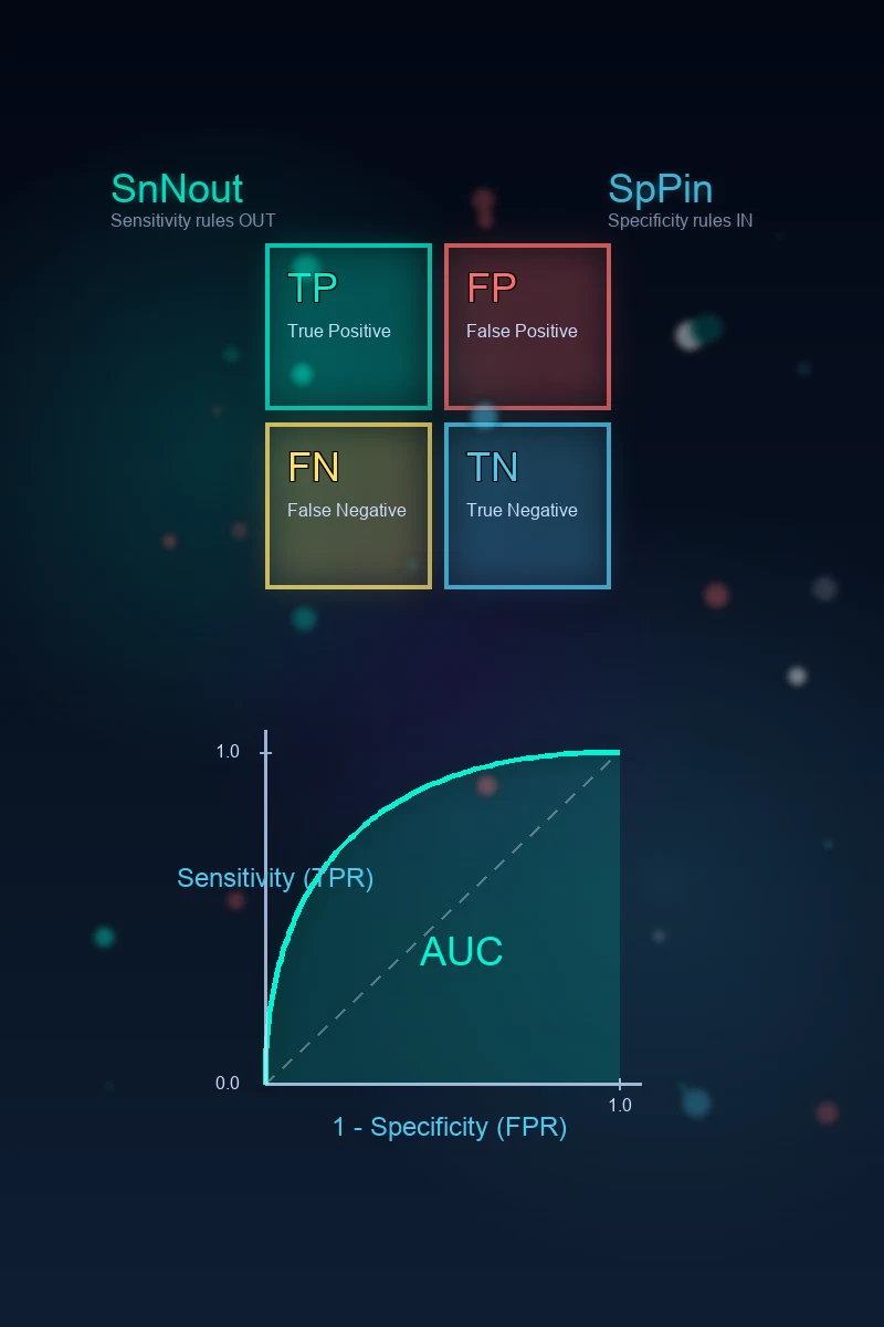
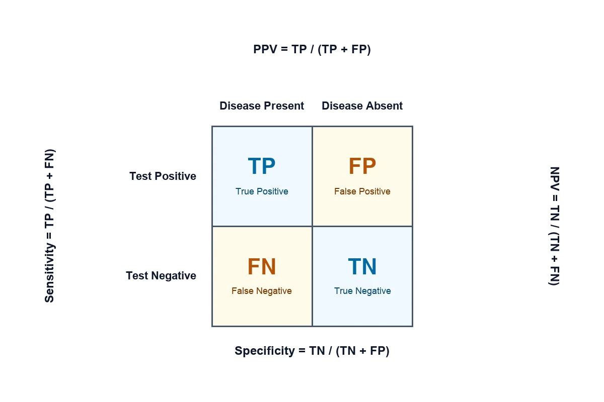
Every metric in this topic is derived from a single object — the 2x2 contingency table that cross-classifies a sample of patients by their true disease status (columns) against their test result (rows). The four cells are: [1]

• True positives (TP) — patients WITH disease in whom the test is POSITIVE (the test is right).
• False positives (FP) — patients WITHOUT disease in whom the test is POSITIVE (a false alarm).
• False negatives (FN) — patients WITH disease in whom the test is NEGATIVE (a missed case).
• True negatives (TN) — patients WITHOUT disease in whom the test is NEGATIVE (the test is right). [1]

The columns are defined by the reference standard (the best-available method of establishing the truth — angiography for coronary disease, surgical findings for endometriosis, a composite outcome for major adverse cardiac events). The rows are defined by the index test under evaluation. Sensitivity and specificity are computed down the columns (they condition on disease status), while the predictive values are computed across the rows (they condition on the test result). Getting this orientation right is the single most reliable way to avoid the most common exam error, which is quoting the wrong denominator. The whole topic is, in effect, an elaboration of these four cells and the ratios that connect them [7].

Sensitivity

Sensitivity (Sn), also called the true positive rate or detection rate, is the proportion of patients WITH disease who test POSITIVE. The formula is: [1]

Sensitivity equals TP divided by (TP plus FN). [1]

Read the denominator carefully — it is everyone who truly has the disease (TP plus FN), so sensitivity conditions on disease, not on the test. It answers the question: "If the patient genuinely has the disease, what is the chance the test will catch it?" A sensitivity of 0.90 means the test detects 90 percent of diseased patients and misses 10 percent (the false negatives). Because the calculation uses only the disease column, sensitivity is a fixed property of the test and does not depend on disease prevalence — it travels with the test from the validation study to any population. A highly sensitive test, when negative, makes disease unlikely, which gives the mnemonic SnNout — a SENSITIVE test, NEGATIVE, rules OUT. The clinical use of a sensitive test is therefore exclusion: D-dimer to exclude PE, a highly sensitive troponin to exclude myocardial injury, HIV screening to exclude infection. The iridocorneal-angle AI classification study illustrates how sensitivity is reported for an automated diagnostic: the proportion of truly closed angles the algorithm correctly flags [1].

Specificity

Specificity (Sp), also called the true negative rate, is the proportion of patients WITHOUT disease who test NEGATIVE. The formula is: [1]

Specificity equals TN divided by (TN plus FP). [1]

The denominator is everyone who truly does NOT have the disease (TN plus FP), so specificity, like sensitivity, conditions on disease status. It answers: "If the patient genuinely does not have the disease, what is the chance the test will correctly say so?" A specificity of 0.95 means that 95 percent of disease-free patients test negative and 5 percent produce a false alarm. Specificity is prevalence-independent for the same reason sensitivity is — the calculation is confined to a single column of the table. A highly specific test, when positive, makes disease likely, which gives the mnemonic SpPin — a SPECIFIC test, POSITIVE, rules IN. The clinical use of a specific test is therefore confirmation: a biopsy to confirm a malignancy flagged on imaging, coronary angiography to confirm ischaemia, or a Western blot to confirm HIV. The gadoxetate-MRI diagnostic-value study reports specificity as the proportion of disease-free patients correctly classified by the imaging test [2].

Positive and negative predictive values

Sensitivity and specificity describe the test. The clinician at the bedside faces the inverse question: the test is positive (or negative) — what is the probability the patient actually has the disease? That is the domain of the predictive values. [1]

• Positive predictive value (PPV) equals TP divided by (TP plus FP) — the proportion of patients with a POSITIVE test who truly have disease. It is read across the positive-test row.
• Negative predictive value (NPV) equals TN divided by (TN plus FN) — the proportion of patients with a NEGATIVE test who truly do not have disease. It is read across the negative-test row. [1]

The defining feature of the predictive values — and the source of most clinical errors in their use — is that they depend on disease prevalence. In a high-prevalence population most positives are true positives and the PPV rises; in a low-prevalence population even a specific test generates false positives that swamp the true positives, and the PPV falls. The AI-CT study for major adverse cardiac events is a clear illustration: a CT-based risk flag with modest specificity generates a high PPV in a high-risk vascular surgical cohort but a low PPV in a young, low-risk day-case population, because the baseline event rate (the prevalence) is so different. NPV moves in the opposite direction — as prevalence rises, NPV falls, because a negative test leaves more residual risk. This is the core reason a test validated in an ICU cannot be transplanted unchanged into a screening clinic [5].

Prevalence and Bayes' theorem

The dependence of the predictive values on prevalence is the clinical face of Bayes' theorem, which states that the post-test probability of disease is a function of the pre-test probability (the prevalence in the patient's population, modified by the clinical picture) and how much the test result shifts that probability. Formally, in odds form: [1]

Post-test odds equals pre-test odds times the likelihood ratio. [1]

The pre-test odds are derived from the pre-test probability (prevalence); the likelihood ratio, described next, is the weight the test result carries. The practical implication is that the same test result means different things in different patients. A positive D-dimer in a young, immobilised patient with pleuritic chest pain (high pre-test probability) substantially raises the probability of PE and warrants imaging; a positive D-dimer in an asymptomatic outpatient (low pre-test probability) may reflect nothing and requires no further action. The regional-versus-general-anaesthesia meta-analysis is an example of how the baseline risk of the population determines how an intervention's apparent effect should be interpreted — the same principle of baseline probability that Bayes' theorem formalises for a diagnostic test [8].

Likelihood ratios

The likelihood ratios combine sensitivity and specificity into a single number that, crucially, does not depend on prevalence — and so travels intact from the validation population to any individual patient. There are two: [1]

• LR+ (positive test) equals sensitivity divided by (1 minus specificity) — how many times more likely a positive result is in a diseased than a non-diseased person.
• LR- (negative test) equals (1 minus sensitivity) divided by specificity — how many times less likely a negative result is in a diseased than a non-diseased person. [1]

The interpretation is by magnitude. An LR+ greater than 10 is very useful — it multiplies the pre-test odds by more than ten and substantially raises the probability of disease. An LR- less than 0.1 is very useful in the other direction — it divides the pre-test odds by more than ten and substantially lowers the probability of disease. Values near 1.0 carry no useful information. Because the likelihood ratios are prevalence-independent, they are the preferred vehicle for moving a test from a study to a bedside: take the patient's pre-test probability (the prevalence in their clinical context), convert it to pre-test odds, multiply by the LR for the result you observed, and convert back to a post-test probability — that is Bayes' theorem in operational form. The deep-learning glaucoma referral study reports likelihood ratios as part of its diagnostic-accuracy profile, illustrating how LRs characterise a test's ability to move probability across the spectrum of disease [4].

ROC curves

The receiver operating characteristic (ROC) curve is the master plot of diagnostic test performance. It plots sensitivity (true positive rate) on the y-axis against (1 minus specificity) (the false positive rate) on the x-axis for every possible threshold of the test. A test that separates diseased from non-diseased perfectly traces a curve that rises steeply to the top-left corner; a test that carries no information sits on the diagonal. [1]

The area under the curve (AUC) summarises overall discrimination in a single number: [1]

• AUC equals 0.5 — the test is no better than chance (the diagonal).
• AUC equals 1.0 — the test is perfect.
• AUC greater than 0.9 — excellent discrimination.
• AUC of 0.7 to 0.8 — acceptable; 0.8 to 0.9 — good. [1]

The AUC is the probability that, given one randomly chosen diseased patient and one randomly chosen non-diseased patient, the test assigns a higher score to the diseased one. Two tests can be compared by comparing their AUCs. The ROC curve also makes the threshold trade-off visible: moving the threshold left raises sensitivity and lowers specificity (moving up and to the right along the curve), while moving it right does the reverse. The iridocorneal-angle AI classification and the glaucoma-referral studies both report AUCs as the headline measure of their algorithms' performance, and reading those numbers critically is now part of the anaesthetist's task when an AI tool is deployed in perioperative care [1][4].

Choosing a diagnostic threshold

A continuous test has no single "positive" cut-off — the threshold is a choice, and the choice depends on the clinical purpose. The ROC curve makes the trade-off explicit, and the clinical context dictates where on the curve to operate. [1]

• High-sensitivity setting (screening). When missing a case is dangerous and the consequences of a false positive are acceptable, set the threshold low so that almost every diseased patient tests positive. Screening for HIV, a lactate threshold to flag sepsis, and D-dimer to exclude PE all use high-sensitivity thresholds; the price is more false positives, who then undergo a specific confirmatory test. The cerebral-autoregulation algorithm study illustrates how an alerting threshold is tuned to detect nearly every episode of autoregulation failure, accepting that some alerts will be false [3].
• High-specificity setting (confirmation). When a false positive would trigger harmful or irreversible action — an unnecessary biopsy, an invasive angiogram, a lifetime of label and treatment — set the threshold high so that almost every positive result is a true positive. Biopsy confirms a malignancy flagged on imaging; coronary angiography confirms ischaemia; a Western blot confirms HIV.

The same test can therefore be operated at different thresholds for different purposes: a troponin assay run at a high-sensitivity threshold to rule out myocardial injury in the emergency department, and at a higher rule-in threshold to confirm a type 1 myocardial infarction. The threshold is a clinical decision, not a property of the assay. [1]

Applied examples in anaesthesia

The framework comes alive in the tests anaesthetists use every day. [1]

• D-dimer for PE exclusion. D-dimer has high sensitivity but low specificity — it catches almost every PE (a negative result usefully rules out) but is elevated by inflammation, pregnancy, surgery and malignancy, so most positives are not PE. Its role is therefore exclusion, not diagnosis; a positive D-dimer prompts imaging, it does not diagnose PE.
• High-sensitivity troponin for perioperative MI. Modern assays detect tiny rises in troponin, giving high sensitivity at the cost of low specificity (any myocardial injury — sepsis, heart failure, renal failure — raises troponin). The predictive value of a positive troponin in a low-risk asymptomatic postoperative patient is therefore modest, which is why perioperative myocardial injury is defined by a threshold rather than by a single "positive" value.
• Mallampati score for difficult airway prediction. Mallampati has both low sensitivity AND low specificity, which is why it poorly predicts difficult laryngoscopy: most "high-grade" scores are followed by straightforward intubations (low PPV), and many genuinely difficult airways are not flagged (low sensitivity). It is a screening cue, not a diagnostic test, and is combined with other predictors precisely because no single test performs adequately alone.
• FAST scan for trauma. FAST has high specificity for intra-abdominal free fluid in the unstable trauma patient (a positive scan prompts laparotomy) but limited sensitivity — a negative FAST does not exclude injury in a stable patient, who still warrants CT. The threshold for action is set by haemodynamics, not by the scan alone. [1]

These examples share a common thread: the test's role is determined by which of its properties — sensitivity or specificity — the clinical question exploits, and by how the local prevalence shapes the predictive value [6][8].

Evaluating a new diagnostic test

A new test (especially an AI tool) is evaluated by comparing it against a reference standard — the best-available method of establishing the truth — in an appropriate sample of patients, and reporting the comparison under the STARD guidelines (Standards for Reporting of Diagnostic Accuracy Studies), which specify the flow of patients, the index test, the reference standard, and the 2x2 table. Three biases distort the apparent performance: [1]

• Spectrum bias. If the validation population contains only severe disease and healthy controls, the test looks artificially accurate; the spectrum does not match the indeterminate patients in whom the test will actually be used. A test validated in a tertiary ICU may perform poorly in a primary-care population.
• Verification bias (work-up bias). If only patients with a positive index test undergo the reference standard (because it is invasive or expensive), the false negatives are systematically missed and both sensitivity and specificity appear inflated. Correct design verifies a representative sample regardless of the index test result.
• **Reference standard bias.**If the reference standard is itself imperfect, the apparent accuracy of the index test is bounded by the accuracy of the reference. [1]

The gadoxetate-MRI and bladder-endometriosis diagnostic studies are examples of work in which the index test is measured against a defined reference standard, and reading them critically means checking that the spectrum matches your patients and that verification was not conditional on the test result [2][6].

Screening versus diagnostic testing

The final distinction is between screening and diagnostic testing, and it determines how a test is deployed. [1]

• Screening is applied to an asymptomatic population at risk of a disease. The priority is high sensitivity — do not miss cases — and false positives are tolerated because the next step is a specific confirmatory test. Examples include HIV screening, mammography, and anaesthetic preoperative risk stratification. Because the population is asymptomatic the prevalence is low, so even a specific test has a low PPV, which is why a positive screen is never the end of the pathway.
• Diagnostic testing is applied to a symptomatic patient (or one with an abnormal screen) in whom disease is already suspected. The priority is high specificity — confirm the diagnosis and avoid false alarms that would trigger harmful intervention — and the higher prevalence in this group raises the PPV. [1]

The glaucoma-referral AI is a screening application (it must not miss referable disease in an asymptomatic population, so it is tuned for sensitivity, and false referrals are worked up by an ophthalmologist), whereas the AI-CT for MACE operates closer to a diagnostic role in a symptomatic, higher-risk cohort [4][7].

[1] [1]

Red flags

[1]

References

1. [1]Rubegni G, et al. Automated iridocorneal angle classification using a multimodal large language model Graefes Arch Clin Exp Ophthalmol, 2026.PMID 42363984
2. [2]Sandrasegaran K, et al. Do hepatic and biliary functional data from gadoxetate-enhanced MRI add value in predicting outcomes in primary sclerosing cholangitis (PSC)? Eur Radiol, 2026.PMID 42363965
3. [3]Albanese A, et al. A Novel Algorithm for Continuous Real-Time Cerebral Autoregulation Assessment Based on Mean Arterial Pressure and Cerebral Oxygen Saturation Anesth Analg, 2026.PMID 42363900
4. [4]Lima-Cabrita A, et al. Deep learning in glaucoma referral: Performance assessment using a real-world setting Acta Ophthalmol, 2026.PMID 42363827
5. [5]Xu T, et al. The diagnostic and predictive value of AI-combined multilayer spiral CT for MACE after emergency PCI in STEMI patients: A prospective cohort study Medicine (Baltimore), 2026.PMID 42363530
6. [6]Ozdemir BG, et al. Bladder endometriosis: a current overview of pathogenesis, diagnosis, and treatment approaches Abdom Radiol (NY), 2026.PMID 42364038
7. [7]Li JZ, et al. Generative AI in healthcare: redefining clinical practice through digital transformation Health Econ Rev, 2026.PMID 42364007
8. [8]Li P, et al. Regional versus general anesthesia for femur and hip fracture surgery: A meta-analysis of postoperative outcomes and complications J Int Med Res, 2026.PMID 42363795