ICU · Statistics & evidence-based medicine
Diagnostic Tests — Sensitivity, Specificity, Predictive Values, Likelihood Ratios & ROC
Also known as Diagnostic tests · Sensitivity · Specificity · Positive predictive value · Likelihood ratio · ROC curve · SnNout SpPin · Fagan's nomogram · Bayes theorem · Number needed to diagnose
Diagnostic test properties for the ICU First Part: the 2x2 table; sensitivity (SnNout) and specificity (SpPin) as intrinsic test properties; positive and negative predictive values that depend on prevalence; likelihood ratios (LR+ and LR-) that combine with pre-test probability via the Bayesian odds form and Fagan's nomogram; the ROC curve and its area under the curve as a measure of discrimination; the Youden index and number needed to diagnose; and worked examples for D-dimer in suspected PE and high-sensitivity troponin in suspected MI.
On this page & tools
Your progress
Saved locally on this device.
Target exams
Overview
A diagnostic test is judged against a reference ("gold") standard. The results form a 2x2 table of true and false, positive and negative results, from which the test's properties are derived. Sensitivity and specificity describe the test itself; predictive values depend on how common the disease is; and likelihood ratios combine test performance with clinical pre-test probability through the Bayesian (odds) form of Bayes' theorem. The whole framework rests on the recognition that no test is purely "positive" or "negative" in isolation - its meaning is always a function of the patient in front of you.[1][7]


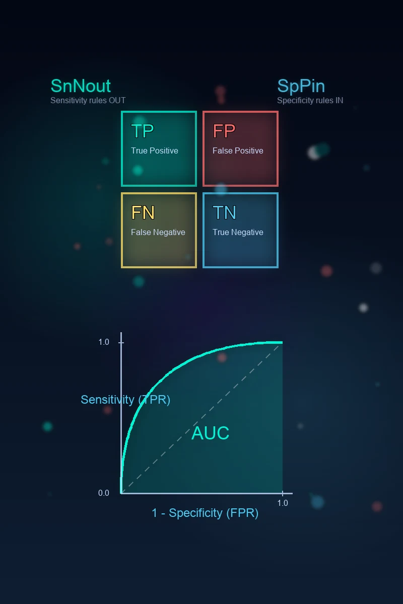
The 2x2 table
The foundation of every diagnostic-test calculation is the 2x2 (contingency) table, which cross-tabulates the test result against the (independently verified) gold-standard truth:[7]
| Disease present | Disease absent | Row totals | |
|---|---|---|---|
| Test positive | True positive (TP) | False positive (FP) | TP + FP |
| Test negative | False negative (FN) | True negative (TN) | FN + TN |
| Column totals | TP + FN | FP + TN | N |
Four derived counts matter for every ratio below:[7]
- True positive (TP) - the test is positive and the patient has the disease.
- False positive (FP) - the test is positive but the patient is disease-free (a Type I diagnostic error).
- False negative (FN) - the test is negative but the patient has the disease (a Type II diagnostic error, often the more dangerous).
- True negative (TN) - the test is negative and the patient is disease-free.[7]
Every metric in diagnostic testing is a rearrangement of these four cells. Learn the cells, and the equations fall out of them rather than from rote memory.[7]
Sensitivity and specificity (intrinsic to the test)
- Sensitivity = TP / (TP + FN): the proportion of diseased people the test correctly flags. Also called the true-positive rate (TPR) or recall. A highly sensitive test, when negative, rules disease out (SnNout).[1][8]
- Specificity = TN / (TN + FP): the proportion of healthy people the test correctly excludes. Also called the true-negative rate. A highly specific test, when positive, rules disease in (SpPin).[1][8]
- These are properties of the test (and the chosen cut-off) and do not change with disease prevalence. They are estimated from a cohort of patients with known disease status.[1]
Why the mnemonics hold
SnNout (Sensitive test, Negative result, rules OUT disease) is true because a sensitive test has very few false negatives - so a negative result means the patient almost certainly does not have the disease. SpPin (Specific test, Positive result, rules IN disease) is true because a specific test has very few false positives - so a positive result almost certainly reflects true disease. These mnemonics only hold when sensitivity or specificity is very high (typically > 95 per cent); with lower values the predictive-value/likelihood-ratio framework is more honest.[8]
Predictive values (depend on prevalence)
- Positive predictive value (PPV) = TP / (TP + FP): the chance that a positive test is a true positive. It answers the bedside question: "my patient's test is positive - do they have the disease?"
- Negative predictive value (NPV) = TN / (TN + FN): the chance that a negative test is a true negative. It answers: "my patient's test is negative - are they disease-free?"
- Both rise or fall with disease prevalence: a positive test is far more likely to be true when the disease is common (high PPV), and a negative test is more reassuring when the disease is rare (high NPV). This is why a test's behaviour differs between a low-prevalence screening setting and a high-prevalence ICU.[1]
The prevalence dependence, made explicit
Prevalence (pre-test probability, p) determines the column totals in the 2x2 table: TP + FN = p x N and FP + TN = (1 - p) x N. Because PPV and NPV both have a prevalence-dependent cell in their denominator, they swing dramatically with prevalence. Likelihood ratios (below) were invented precisely to escape this dependence.[8]
| Setting | Prevalence | Sensitivity 0.97, Specificity 0.40 (typical D-dimer for PE) | PPV | NPV |
|---|---|---|---|---|
| Primary care screening | 5 per cent | TP 48.5 / FN 1.5 / FP 570 / TN 380 | 7.8 per cent | 99.6 per cent |
| ED, chest pain / dyspnoea | 20 per cent | TP 194 / FN 6 / FP 480 / TN 320 | 28.8 per cent | 98.2 per cent |
| ICU, haemodynamically unstable | 50 per cent | TP 485 / FN 15 / FP 300 / TN 200 | 61.8 per cent | 93.0 per cent |
Note how the same test (identical sensitivity and specificity) yields a PPV ranging from under 8 per cent to over 60 per cent purely by changing the population tested. This is the single most important concept in diagnostic testing and the most common viva trap.[1][8]
Likelihood ratios (combine test and clinical probability)
- LR+ = sensitivity / (1 - specificity) = the true-positive rate divided by the false-positive rate. It answers: "how many times more likely is a positive test in a diseased than a non-diseased person?"
- LR- = (1 - sensitivity) / specificity = the false-negative rate divided by the true-negative rate. It answers: "how many times less likely is a negative test in a diseased than a non-diseased person?"
- Likelihood ratios are independent of prevalence and combine with the pre-test probability (via odds) to give a post-test probability - useful because they let you apply one test's performance to your specific patient's clinical context. An LR+ above 10 (or LR- below 0.1) generates a large, often conclusive shift in probability; LR+ of 5-10 (LR- of 0.1-0.2) is moderate; LR+ of 2-5 (LR- of 0.2-0.5) is small and rarely useful alone.[1][8]
Interpreting the magnitude of a likelihood ratio
| LR+ | LR- | Strength of evidence the test provides |
|---|---|---|
| > 10 | < 0.1 | Large, often conclusive shift in probability |
| 5 - 10 | 0.1 - 0.2 | Moderate shift |
| 2 - 5 | 0.2 - 0.5 | Small, rarely enough alone |
| 1 - 2 | 0.5 - 1 | Very small, rarely important |
| 1.0 | 1.0 | No information at all (the test result is equally likely sick or well) |
An LR of exactly 1 means the test result carries no diagnostic information - a sobering reminder that a "normal" result on a useless test changes nothing.[8]
The Bayesian approach — pre-test and post-test probability
Diagnostic reasoning is fundamentally Bayesian: you begin with a pre-test probability (your clinical estimate of disease likelihood before the test), apply the test's result through its likelihood ratio, and arrive at a post-test probability. The mechanism is the odds form of Bayes' theorem:[8]
Post-test odds = Pre-test odds x Likelihood ratio[8]
where the conversion between probability and odds is:[4]
- Odds = probability / (1 - probability)
- Probability = odds / (1 + odds)[4]
Worked example of the Bayesian calculation
Suppose your patient has a 15 per cent pre-test probability of pulmonary embolism (a moderate Wells score) and the D-dimer returns positive (LR+ of 1.6 for a conventional D-dimer):[4]
- Pre-test odds = 0.15 / (1 - 0.15) = 0.176.
- Post-test odds = 0.176 x 1.6 = 0.282.
- Post-test probability = 0.282 / (1 + 0.282) = 0.220 (22 per cent).[4]
A positive D-dimer in a moderate-probability patient has lifted the probability only from 15 to 22 per cent - still below the imaging threshold, which is exactly why a positive D-dimer alone never "rules in" PE. Run the same numbers with the D-dimer negative (LR- 0.08):[4]
- Post-test odds = 0.176 x 0.08 = 0.0141.
- Post-test probability = 0.0141 / 1.0141 = 0.014 (1.4 per cent).[4]
A negative D-dimer collapses the probability below the 1-2 per cent test threshold at which further imaging is safely withheld - the whole basis of the PERC and Wells-D-dimer pathways.[2][3]
Fagan's nomogram
Fagan's nomogram (Fagan, 1975) is the graphical device that performs the Bayesian odds calculation without arithmetic. It is a three-axis diagram:[8]
- The left axis is the pre-test probability (0-100 per cent).
- The middle axis is the likelihood ratio (on a log scale).
- The right axis is the post-test probability (0-100 per cent).[4]
You draw a straight line from your pre-test probability on the left, through the likelihood ratio of the test result in the middle, and read off the post-test probability on the right. The nomogram is a physical embodiment of Bayes' theorem: a high LR+ steepens the line upward toward certainty, a low LR- drives it down toward exclusion, and an LR near 1 leaves the line nearly horizontal (the test has changed nothing).[8]
The power of the nomogram is that it makes explicit what is too often implicit: a test result only moves you from where you already are. A brilliant LR+ applied to an absurdly low pre-test probability still yields a low post-test probability, and a powerful LR- applied to an absurdly high pre-test probability still leaves disease likely. This is why anchoring the pre-test probability (the clinical gestalt, the Wells or PERC score, the bedside sonography) is as important as the test itself.[4]
Applying Bayes' theorem at the bedside — the four-step discipline
Estimate the pre-test probability
Anchor disease likelihood on the clinical picture, validated scores (Wells, PERC, GRACE), and local prevalence. Resist anchoring on a single dramatic feature. State the probability as a number (e.g. 15 per cent), not a vague "low/moderate/high".
Choose a test whose LR you know
Look up the likelihood ratio for the result you actually got in a setting comparable to yours (spectrum, cut-off). LRs travel better than PPV/NPV because they are prevalence-independent, but they still depend on the test being applied to a similar patient spectrum.
Apply the Bayesian odds form
Post-test odds = pre-test odds x LR. Convert pre-test probability to odds, multiply, convert back. Equivalently, draw a straight line on Fagan's nomogram from pre-test probability through the LR to the post-test probability.
Decide against a threshold
Compare the post-test probability to your test-treatment threshold: below it (typically below 1-2 per cent for PE), stop and reassure; above the treatment threshold, treat; in between, do the next test (CTPA, ultrasound, angiography). The threshold, not the number, drives the decision.
Worked example 1 — D-dimer for suspected pulmonary embolism
The D-dimer is the archetype of a high-sensitivity, low-specificity test used to rule disease out. A conventional quantitative D-dimer at the usual 500 ug/L cut-off has a sensitivity of roughly 97 per cent and a specificity of roughly 40 per cent for venous thromboembolism.[2][4]
The 2x2 table (in a hypothetical ED cohort of 1000 patients with a 20 per cent PE prevalence - a typical chest-pain/dyspnoea population):[2]
| PE present | PE absent | ||
|---|---|---|---|
| D-dimer positive | TP 194 | FP 480 | 674 |
| D-dimer negative | FN 6 | TN 320 | 326 |
| 200 | 800 | 1000 |
Derived metrics:[2]
- Sensitivity = 194 / 200 = 97.0 per cent (SnNout: a negative D-dimer is reassuring).
- Specificity = 320 / 800 = 40.0 per cent (a positive D-dimer is unhelpful for ruling in - SpPin fails).
- PPV = 194 / 674 = 28.8 per cent (a positive D-dimer in this population means PE in fewer than one in three).
- NPV = 320 / 326 = 98.2 per cent (a negative D-dimer makes PE very unlikely).
- LR+ = 0.97 / 0.60 = 1.62 (small - barely shifts probability upward).
- LR- = 0.03 / 0.40 = 0.075 (large - collapses probability downward).
- Number needed to diagnose = 1 / (0.97 + 0.40 - 1) = 1 / 0.37 = 2.7.[2]
The clinical lesson: a D-dimer is a rule-out test. The negative result (low LR-) is powerful; the positive result (low LR+) is nearly useless for ruling in. This is why every PE pathway gates the D-dimer behind a low or moderate pre-test probability (Wells / PERC) and never acts on a positive D-dimer alone - a positive D-dimer simply mandates imaging.[2][6]
The age-adjusted D-dimer and ADJUST-PE
Because D-dimer rises with age, the fixed 500 ug/L cut-off generates an unacceptably high false-positive rate in older patients, driving over-investigation. The ADJUST-PE trial validated an age-adjusted cut-off (age x 10 ug/L for patients over 50) and showed it safely ruled out PE in a far higher proportion of older patients without an excess of missed PE during three-month follow-up.[5]
Wells et al. — Excluding PE at the bedside without diagnostic imaging (PMID 11453709)
Kline et al. — The PERC rule (PMID 15304025)
van Belle et al. — The Christopher rule (PMID 16403929)
Righini et al. — ADJUST-PE, the age-adjusted D-dimer (PMID 24643601)
Worked example 2 — high-sensitivity troponin for suspected myocardial infarction
The high-sensitivity cardiac troponin (hs-cTn) is the paradigm of a test that can both rule in and rule out, because its sensitivity and specificity are both high. At 3 hours from presentation, a typical hs-cTnT assay has a sensitivity of roughly 95 per cent and a specificity of roughly 85 per cent for type 1 myocardial infarction.[10][11]
The 2x2 table (in a hypothetical ED cohort of 1000 patients with chest pain and a 15 per cent prevalence of NSTEMI):[10]
| MI present | MI absent | ||
|---|---|---|---|
| hs-cTn positive | TP 143 | FP 128 | 271 |
| hs-cTn negative | FN 7 | TN 722 | 729 |
| 150 | 850 | 1000 |
Derived metrics:[10]
- Sensitivity = 143 / 150 = 95.3 per cent.
- Specificity = 722 / 850 = 84.9 per cent.
- PPV = 143 / 271 = 52.8 per cent (a positive troponin means MI in just over half).
- NPV = 722 / 729 = 99.0 per cent (a negative troponin at 3 h makes MI very unlikely).
- LR+ = 0.953 / 0.151 = 6.3 (moderate - meaningful for rule-in).
- LR- = 0.047 / 0.849 = 0.06 (large - powerful for rule-out).
- Number needed to diagnose = 1 / (0.953 + 0.849 - 1) = 1 / 0.802 = 1.2.[10]
The clinical lesson: unlike D-dimer, hs-cTn has both a useful LR+ and a useful LR-, so it can both rule out (low LR-) and meaningfully raise suspicion (useful LR+). This dual utility is why modern pathways (the ESC 0/1-hour and 0/2-hour algorithms) build the troponin delta into the rule-in/rule-out decision rather than treating a single threshold as binary.[10][11]
Why troponin "positives" are often not MI
Despite a respectable specificity, troponin rises in a long list of non-MI conditions - sepsis, renal failure, heart failure, pulmonary embolism (right-ventricular strain), myocarditis, tachyarrhythmias, stroke, and critical illness itself. A single elevated troponin is therefore a "specific test" only in a population without these competing causes; in the ICU, where troponin-elevating illness is the rule, the test's operational specificity collapses. This is the spectrum effect in action: a test's measured performance depends on the sort of patient it is applied to.[1]
Applying a high-sensitivity troponin in suspected MI — the ESC 0/1-hour pathway
Estimate pre-test probability
Combine chest-pain characteristics, risk factors, ECG findings (is there ST-elevation, ST-depression, T-wave inversion?) and bedside findings. STEMI is a clinical + ECG diagnosis - do not wait for troponin to activate the catheter lab.
Draw hs-cTn at presentation and again at 1 hour
Use a validated assay-specific algorithm (ESC 0/1-hour). The absolute value AND the delta (change between the two) together define rule-in and rule-out zones.
Rule OUT if both values are very low and the delta is small
A presentation value below the limit of detection with a sub-threshold 1-hour delta safely rules out NSTEMI in most patients and allows safe early discharge. This is the high-NPV / low-LR- limb in action.
Rule IN if the value or delta crosses the high zone
A high absolute value or a large 1-hour delta rules in NSTEMI - admit and pursue the ACS pathway (antiplatelet, anticoagulant, early invasive strategy as appropriate).
If in the observational zone, continue
A substantial minority fall between the rule-in and rule-out cut-offs - repeat troponin at 2-3 hours, look for a rise/fall pattern, and integrate serial ECGs and clinical assessment before deciding.
Number needed to diagnose (NND)
The number needed to diagnose (NND) is the diagnostic analogue of the number needed to treat. It answers: "how many patients do I have to test to find one true positive that I would not have found by chance?" It is defined via the Youden index:[8]
NND = 1 / (sensitivity + specificity - 1) = 1 / Youden index[10]
where the Youden index J = sensitivity + specificity - 1 ranges from 0 (useless test) to 1 (perfect test).[10]
Examples
- D-dimer for PE (sens 0.97, spec 0.40): J = 0.37, NND = 2.7 - you need to test fewer than three patients to find one extra true positive over chance. This looks efficient but is misleading, because the test's specificity is so low that most "positives" are false.
- hs-cTn for MI (sens 0.95, spec 0.85): J = 0.80, NND = 1.2 - a far more discriminating test.
- A useless test (sens 0.50, spec 0.50): J = 0, NND is infinite - the test provides no information.[3]
The NND is a useful summary statistic for comparing tests, but like the AUC it hides the cut-off trade-off: a test with a high Youden index at one cut-off may still be a poor rule-out (or rule-in) tool in practice. The likelihood-ratio framework remains the bedside truth.[8]
The ROC curve and its area
- A receiver operating characteristic (ROC) curve plots sensitivity (true-positive rate) against 1 - specificity (false-positive rate) across all cut-off values. A test that discriminates perfectly bows to the top-left corner; a useless test lies on the diagonal.[9]
- The area under the curve (AUC) summarises discrimination: 0.5 is no better than chance, 1.0 is perfect. An AUC of about 0.8 represents a good test; 0.9 or above is excellent.[9]
- The Youden index picks the cut-off that maximises (sensitivity + specificity - 1) - the point on the ROC curve furthest from the diagonal. This is the "best overall" cut-off, but it may not be the cut-off you want clinically (a rule-out cut-off moves left to maximise sensitivity; a rule-in cut-off moves right to maximise specificity).
Reading the ROC curve
| AUC | Interpretation |
|---|---|
| 0.5 | No discrimination (equivalent to flipping a coin) |
| 0.7 - 0.8 | Acceptable / fair discrimination |
| 0.8 - 0.9 | Good discrimination |
| > 0.9 | Excellent discrimination |
| 1.0 | Perfect discrimination |
The ROC curve's great value is that it displays the cut-off trade-off visually: every point on the curve is a possible threshold, and the clinician (or guideline) chooses the one that fits the clinical question - a sensitive cut-off (upper-left, high sensitivity) to rule out, a specific cut-off (lower-right, high specificity) to rule in. Two tests can be compared by overlaying their curves: the one bowing further toward the top-left corner has the greater AUC and the better overall discrimination.[9]
Hanley & McNeil — The meaning and use of the area under a ROC curve (PMID 7063747)
The spectrum effect and other biases in diagnostic accuracy studies
A test's reported sensitivity and specificity are estimates, and they are vulnerable to systematic error at the study-design level. The four classic biases to name in the viva:[7]
- Spectrum bias arises when the study population does not represent the patients the test will be used on - e.g. measuring a troponin assay's specificity in healthy blood donors rather than in dyspnoeic, septic ICU patients who have competing causes of troponin elevation. The measured specificity will be falsely reassuring.
- Verification (work-up) bias arises when only positive (or only negative) tests are confirmed by the gold standard - the test's apparent accuracy is inflated because the truth was never established in the patients most likely to expose its errors.
- Review bias arises when the gold-standard interpretation is contaminated by knowledge of the test result (or vice versa) - the test and the standard must be interpreted blind to each other.
- Incorporation bias arises when the index test is part of the gold-standard definition - e.g. the clinical syndrome that defines disease already incorporates the test being evaluated, artificially inflating its apparent accuracy.[7]
The STARD reporting standard exists precisely to force authors to describe the patients, the reference standard, and the blinding, so that these biases can be judged.[7]
The diagnostic-test properties compared
Sensitivity (intrinsic)
- Sensitivity = TP / (TP + FN) - the true-positive rate.
- A property of the test (and the cut-off); does NOT change with prevalence.
- Mnemonic: SnNout - a Sensitive test, when Negative, rules OUT disease.
- High-sensitivity tests (D-dimer, hs-cTn at presentation) are used to RULE OUT.
- Tells you nothing about a positive result - that is specificity and PPV.
Specificity (intrinsic)
- Specificity = TN / (TN + FP) - the true-negative rate.
- A property of the test (and the cut-off); does NOT change with prevalence.
- Mnemonic: SpPin - a Specific test, when Positive, rules IN disease.
- High-specificity tests (a visible vessel on endoscopy, a fracture on X-ray) are used to RULE IN.
- Tells you nothing about a negative result - that is sensitivity and NPV.
PPV (prevalence-dependent)
- PPV = TP / (TP + FP) - the chance a positive test is true.
- Answers the bedside question: "my test is positive - do they have the disease?"
- RISES with prevalence (a positive test is more often true when disease is common).
- In a low-prevalence population even a specific test generates mostly false positives.
- It is why a positive D-dimer in primary care is almost always a false alarm.
NPV (prevalence-dependent)
- NPV = TN / (TN + FN) - the chance a negative test is true.
- Answers the bedside question: "my test is negative - are they disease-free?"
- FALLS with prevalence (a negative test is less reassuring when disease is common).
- In a high-prevalence population even a sensitive test misses disease.
- It is why a negative D-dimer in a high-Wells-probability patient still mandates imaging.
SAQ — Constructing and interpreting a 2x2 table for a diagnostic test
10 minutes · 10 marks
A new rapid bedside assay for the diagnosis of invasive pulmonary aspergillosis in immunocompromised ICU patients is evaluated against a composite reference standard (histopathology plus galactomannan plus culture). In a prospective study of 400 patients, 80 have proven aspergillosis. The new assay is positive in 70 of the 80 diseased and in 60 of the 320 non-diseased. Construct the 2x2 table and derive the sensitivity, specificity, PPV, NPV, LR+, LR-, and the number needed to diagnose.
SAQ — High-sensitivity troponin in suspected acute coronary syndrome and the ESC 0/1-hour pathway
10 minutes · 10 marks
A 65-year-old man presents to the ED with 2 hours of central chest pain. The ECG shows no ST elevation. The high-sensitivity troponin T (hs-cTnT) at presentation is 25 ng/L (LOD 5 ng/L, 99th percentile 14 ng/L) and at 1 hour is 38 ng/L. Outline the diagnostic approach, the interpretation of the troponin using the ESC 0/1-hour algorithm, and the differential of a non-MI troponin rise.
Clinical pearls — the exam-exhaustive set
The derivation of each metric — a single compact map
To anchor the equations, derive each one from the four cells of the 2x2 table. The denominators tell the story:[10]
Deriving every diagnostic metric from the 2x2 cells
Sensitivity — among the DISEASED
Denominator is the diseased column (TP + FN). Sensitivity = TP / (TP + FN). It answers: of all who truly have the disease, what fraction does the test catch?
Specificity — among the HEALTHY
Denominator is the healthy column (FP + TN). Specificity = TN / (TN + FP). It answers: of all who are truly disease-free, what fraction does the test correctly call negative?
PPV — among the POSITIVE tests
Denominator is the positive-test row (TP + FP). PPV = TP / (TP + FP). It answers: of all positive tests, what fraction are true? The denominator is prevalence-dependent, so PPV swings with prevalence.
NPV — among the NEGATIVE tests
Denominator is the negative-test row (FN + TN). NPV = TN / (TN + FN). It answers: of all negative tests, what fraction are true? Also prevalence-dependent.
LR+ — ratio of true-positive to false-positive rates
LR+ = [TP/(TP+FN)] / [FP/(FP+TN)] = sensitivity / (1 - specificity). It is built from two intrinsic quantities, so it is prevalence-independent.
LR- — ratio of false-negative to true-negative rates
LR- = [FN/(TP+FN)] / [TN/(FP+TN)] = (1 - sensitivity) / specificity. Also prevalence-independent.
Youden index and NND
Youden J = sensitivity + specificity - 1. Number needed to diagnose NND = 1 / J. These summarise overall discrimination but hide the operating point.
AUC — integration across all cut-offs
The area under the ROC curve integrates discrimination across every possible cut-off. It is the probability that the test ranks a random diseased subject above a random healthy one.
Worked Bayesian walk-through — D-dimer across three pre-test probabilities
To make the prevalence dependence visceral, run the same D-dimer (LR+ 1.6, LR- 0.07) through three different patients:[8]
| Pre-test probability | Pre-test odds | If D-dimer POSITIVE (x1.6) | Post-test probability | If D-dimer NEGATIVE (x0.07) | Post-test probability |
|---|---|---|---|---|---|
| 5 per cent (PERC-negative, very low risk) | 0.053 | 0.084 | 7.8 per cent | 0.0037 | 0.4 per cent |
| 20 per cent (Wells moderate) | 0.250 | 0.400 | 28.6 per cent | 0.0175 | 1.7 per cent |
| 60 per cent (Wells high) | 1.500 | 2.400 | 70.6 per cent | 0.105 | 9.5 per cent |
The lesson: in the very-low-risk patient, even a positive D-dimer only raises the probability to ~8 per cent (still imaging territory, but not alarming); in the high-risk patient, even a negative D-dimer leaves a ~10 per cent probability - high enough to mandate imaging regardless. This is why guidelines say: in a high-probability patient, skip the D-dimer and image.[6]
The structured PE rule-out pathway — operationalising Bayes' theorem
Is the patient low-risk by gestalt and haemodynamically stable?
If not (shock, hypotension, profound hypoxia), the pre-test probability is high - go straight to imaging (CT pulmonary angiography) and consider empiric anticoagulation. The D-dimer has no role here.
Apply PERC
In the very-low-risk patient, check all eight PERC criteria. If ALL are negative, the pre-test probability is below the test threshold - stop. No D-dimer, no imaging.
If PERC-positive, apply the Wells score
Quantify the probability (dichotomised Christopher rule: PE unlikely vs PE likely, or three-tier low/moderate/high).
If PE unlikely / low-probability, check D-dimer
Use age-adjusted cut-off (age x 10 ug/L) in patients over 50. A negative D-dimer safely excludes PE. A positive D-dimer mandates imaging - it does NOT diagnose PE.
If PE likely / high-probability, or D-dimer positive, proceed to CTPA
In the unstable patient where CTPA is unsafe, perform bedside echocardiography (right-ventricular strain) and consider thrombolysis on clinical grounds.
Apply the test-treatment threshold
The whole exercise is to decide whether the post-test probability is below the threshold to stop (typically <1-2 per cent for PE) or above it. The D-dimer and the scores are tools for crossing that threshold, not for making the diagnosis.
Sample exam question — the worked answer
[10] [2]Red flags
References
- [1]Karnad DR, Nor MBM, Richards GA, et al. Intensive care in severe malaria: Report from the task force on tropical diseases by the World Federation of Societies of Intensive and Critical Care Medicine. Journal of critical care, 2018.PMID 29132978
- [2]Wells PS, Anderson DR, Rodger M, et al Excluding pulmonary embolism at the bedside without diagnostic imaging: management of patients with suspected pulmonary embolism presenting to the emergency department by using a simple clinical model and D-dimer. Ann Intern Med, 2001.PMID 11453709
- [3]Kline JA, Nelson RD, Jackson RE, et al. Criteria for the safe use of D-dimer testing in emergency department patients with suspected pulmonary embolism: a multicenter US study. Annals of emergency medicine, 2002.PMID 11823768
- [4]van Belle A, Buller HR, Huisman MV, et al (Christopher Study Investigators) Effectiveness of managing suspected pulmonary embolism using an algorithm combining clinical probability and D-dimer testing. JAMA, 2006.PMID 16403929
- [5]Righini M, Van Es J, Den Exter PL, et al (ADJUST-PE Investigators) Age-adjusted D-dimer cutoff levels to rule out pulmonary embolism: the ADJUST-PE study. JAMA, 2014.PMID 24643601
- [6]Konstantinides SV, Meyer G, Becattini C, et al (ESC Task Force) 2019 ESC Guidelines for the diagnosis and management of acute pulmonary embolism. Eur Respir J, 2019.PMID 31473594
- [7]Jaeschke R, Guyatt G, Sackett DL Users' guides to the medical literature. III. How to use an article about a diagnostic test. A. Are the results of the study valid? JAMA, 1994.PMID 8283589
- [8]Jaeschke R, Guyatt GH, Sackett DL Users' guides to the medical literature. III. How to use an article about a diagnostic test. B. What are the results and will they help me in caring for my patients? JAMA, 1994.PMID 8309035
- [9]Hanley JA, McNeil BJ The meaning and use of the area under a receiver operating characteristic (ROC) curve. Radiology, 1982.PMID 7063747
- [10]Reichlin T, Schindler C, Drexler B, et al One-hour rule-out and rule-in of acute myocardial infarction using high-sensitivity cardiac troponin T. Arch Intern Med, 2012.PMID 22892889
- [11]Byrne RA, Rossello X, Coughlan JJ, et al (ESC Task Force) 2023 ESC Guidelines for the management of acute coronary syndromes. Eur Heart J (G Ital Cardiol), 2024.PMID 38291910