ICU · Statistics & evidence-based medicine
Survival Analysis & the Kaplan-Meier Curve
Also known as Survival analysis · Kaplan-Meier · Censoring · Log-rank test · Cox proportional hazards · Hazard ratio · Median survival
Survival analysis for the ICU First Part: time-to-event data and censoring (right-censoring when the event is not observed), the survival function S(t) and its complement the cumulative distribution F(t), the hazard function h(t) and cumulative hazard H(t), the Kaplan-Meier estimator as a non-parametric step function of survival probability (product of conditional probabilities), the median and restricted mean survival time, the log-rank test comparing curves between groups, and Cox proportional-hazards regression yielding a hazard ratio under the assumption of proportional hazards.
On this page & tools
Your progress
Saved locally on this device.
8 MCQs with explanations
Target exams
Overview
Many ICU outcomes are time-to-event: time to death, to extubation, to discharge, to readmission. These data share a feature that ordinary averages cannot handle - censoring - and survival analysis is the set of methods built for them.[1]
The vocabulary of survival data
Survival analysis describes the time elapsed from a defined origin (ICU admission, intubation, randomisation) to an event (death, extubation, discharge, readmission). Three functions are the mathematical core - any one can be derived from the others.[1]
- The survival function S(t) — the probability of being event-free beyond time t: S(t) = P(T > t). At t = 0, S(0) = 1 (everyone starts event-free); as events accumulate S(t) falls towards 0. The Kaplan-Meier curve is an estimate of S(t). The complement F(t) = 1 − S(t) is the cumulative incidence (the probability the event has occurred by t).[1]
- The hazard function h(t) — the instantaneous risk of the event at time t, given survival up to t: h(t) = limit (as Δt→0) of P(t ≤ T < t+Δt | T ≥ t) / Δt. It is a rate (events per unit time), not a probability, and is always ≥ 0. A constant hazard gives an exponential distribution; a hazard that rises then falls gives a bathtub curve.[1]
- The cumulative hazard H(t) — the integral of the hazard up to time t. It links the other two by the identity S(t) = exp(−H(t)), or equivalently H(t) = −ln S(t). This is why a plot of −ln(−ln S(t)) against ln(t) gives a straight line under proportional hazards (see below).[1]
These three are interchangeable: estimate S(t) and you have h(t) and H(t), and vice versa. Examiners expect you to state what each represents in one sentence, and to know that the hazard is a rate while the survival is a probability. [1]
Censoring
- A subject is censored when their event time is not observed - they are lost to follow-up, withdraw, or the study ends before the event occurs (the commonest form, right-censoring).[1]
- Censored subjects contribute information up to the point of censoring but cannot be counted as having had the event. Ignoring them (or treating them as events) biases the estimate; survival methods use the time they were observed without bias.[1]
Types of censoring
Types of censoring in survival data
| Type | What it means | Example in ICU practice | Handling |
|---|---|---|---|
| Right-censoring (commonest) | The event has not yet occurred by the last time the subject was observed | A patient is alive at ICU discharge and lost to the 90-day mortality dataset; follow-up ends at day 30 while the patient is still alive | Standard Kaplan-Meier / Cox handles this directly — the subject is counted in the at-risk set only up to their last event-free time |
| Left-censoring | The event occurred before the observation period began, but the exact time is unknown | A patient transferred in already intubated — the true time of intubation (the origin) is uncertain | Requires specialised methods (left-truncated / interval-censored models); rarely the focus of ICU exam answers |
| Interval-censoring | The event is known to have occurred between two observation times, but not exactly when | A ventilator-associated event detected on a daily screen — it happened sometime between yesterday's and today's check | Interval-censored regression; often approximated by assuming the event time is the midpoint |
| Informative (non-random) censoring | The reason for censoring is related to prognosis — censoring is not independent of the event | Sicker patients withdraw from a rehabilitation trial, or are transferred out and lost precisely because they are deteriorating | Violates the core assumption of non-informative censoring and biases KM; report censoring patterns and consider sensitivity analyses |
The unspoken assumption behind every Kaplan-Meier curve and Cox model is that censoring is non-informative - a censored subject has the same future risk as a subject still under observation. When this fails (sicker patients selectively lost), the curve is biased, and no amount of mathematical sophistication can fix unreported informative censoring.[1]
The Kaplan-Meier estimator
- A non-parametric estimate of the survival probability S(t) at each time point. It is the product of the conditional probabilities of surviving each interval: at each event time, multiply by (1 minus the number of events divided by the number at risk).[1]
- It produces a step function that drops at each event and is flat between events; censored subjects are marked with small ticks and removed from the at-risk count thereafter.[1]
- The median survival is the time at which the survival curve crosses 0.5 (half the population has had the event) - often a more useful summary than the mean for skewed time-to-event data.[1]
The estimator in symbols
Let $d_t$ be the number of events at time $t$ and $n_t$ the number at risk just before $t$. The Kaplan-Meier estimate is: [1]
Ŝ(t) = ∏ (1 − dᵢ/nᵢ) over all distinct event times tᵢ ≤ t [1]
The product runs only over distinct event times $t_i$ (times at which at least one event occurred). Between event times the estimate does not change — hence the step shape. At each event time the curve steps down by a factor of $(1 - d/n)$; when several events share a time (ties) the drop is correspondingly larger.[1]
A closely related quantity is the Nelson-Aalen estimator of the cumulative hazard, Ĥ(t) = Σ dᵢ/nᵢ (summed over tᵢ ≤ t), from which an alternative survival estimate S̃(t) = exp(−Ĥ(t)) can be formed. The two survival estimates agree closely in moderate-to-large samples; Nelson-Aalen is slightly better when the risk set is small or events are few.[3]
Confidence intervals
Pointwise confidence bands for Ŝ(t) are calculated on the log-log scale (to keep the bounds within 0 and 1) using Greenwood's formula for the variance of the estimator. These are the dotted lines drawn above and below the KM curve. They widen at the tail of the curve, where few subjects remain at risk — which is exactly why the tail of a KM curve is unreliable and should never be over-interpreted.[1]
Worked example — computing a Kaplan-Meier curve from ICU data
Imagine a 10-patient cohort observed for ICU mortality over 14 days. "C" denotes censoring (discharged alive / lost), "D" denotes death. The data, sorted by time: [1]
| Day | At risk just before (n) | Events (d) | Censored | d/n | 1 − d/n | Ŝ(t) after the step |
|---|---|---|---|---|---|---|
| 2 | 10 | 1 (D) | 0 | 0.10 | 0.90 | 1.00 × 0.90 = 0.90 |
| 4 | 9 | 0 | 1 (C) | — | — | 0.90 (no step; censored subject removed) |
| 5 | 8 | 1 (D) | 0 | 0.125 | 0.875 | 0.90 × 0.875 = 0.788 |
| 7 | 7 | 1 (D) | 1 (C) | 0.143 | 0.857 | 0.788 × 0.857 = 0.675 |
| 9 | 5 | 0 | 1 (C) | — | — | 0.675 |
| 11 | 4 | 1 (D) | 0 | 0.25 | 0.75 | 0.675 × 0.75 = 0.506 |
| 14 | 3 | 0 | 3 (end) | — | — | 0.506 |
Reading the curve: S(t) sits at 0.506 at day 14, the curve steps down only on death days (2, 5, 7, 11), and the censored subjects (days 4, 7, 9, 14) would each be marked with a small tick on the step. The median survival here falls just after day 11, where the curve crosses 0.5 (0.506 → estimate ~day 11). Note how a single death at day 11, when only four patients remain at risk, produces a large step (0.675 → 0.506) — this is why the tail of a KM curve is unstable when few are at risk.[1]
Median survival
- Median survival = the smallest time t at which Ŝ(t) ≤ 0.5; read off the KM curve where it crosses the horizontal line at 0.5. Half the population has had the event by this time.[1]
- If the curve never drops to 0.5 (most patients survive the observation window), median survival is not reached and cannot be estimated — a common exam point. In that setting report the survival probability at a fixed time (e.g. "90-day survival was 0.62") instead.[1]
- It communicates intuitively ("half of patients had died by day 28") and, unlike the mean, does not require the entire survival distribution to be known — it is unaffected by censoring after the median, where most data are typically thin.[1]
Restricted mean survival time (RMST)
The mean survival time is, in principle, the area under the survival curve to infinity. But because the right tail is usually censored (and unreliable), the unrestricted mean is rarely estimable. The restricted mean survival time (RMST) solves this by integrating the survival curve only up to a pre-specified time horizon $\tau$: [1]
RMST(τ) = ∫ S(t) dt integrated from time 0 to τ [1]
Geometrically, RMST is the area under the survival curve from time 0 to $\tau$. It is measured in units of time (days, months) and represents the average event-free time enjoyed over that horizon. Between two trial arms, the difference in RMST($\tau$) is a directly interpretable measure of treatment effect ("patients survived an average of 2.4 more days alive over 90 days") — free of the proportional-hazards assumption that Cox regression imposes.[5]
Royston and Parmar argued that RMST is preferable to the hazard ratio when the proportional-hazards assumption is in doubt or when the effect varies over time, because RMST captures the whole curve difference rather than collapsing it into a single ratio. Its weaknesses: it depends on the arbitrary choice of $\tau$ (usually the minimum of the maximum follow-up in each arm), and it loses power when the curves separate late.[5]
Comparing groups
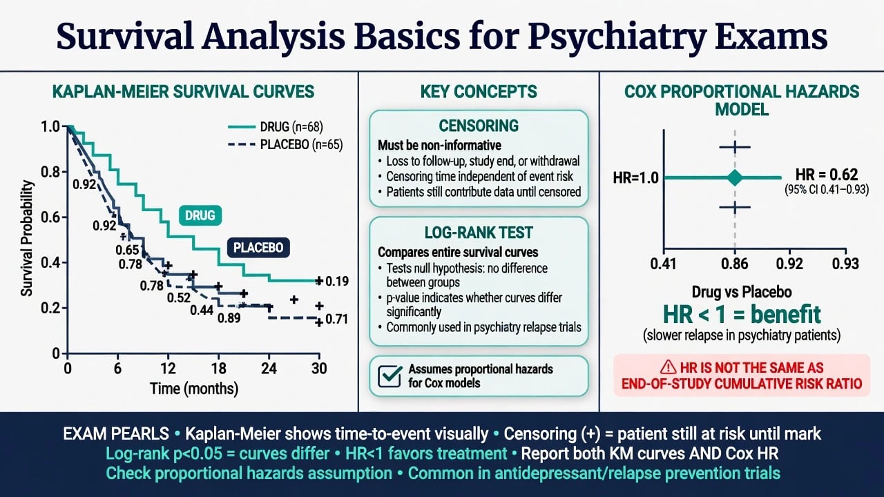
- The log-rank test compares the survival curves of two or more groups non-parametrically, testing whether they differ significantly. It does not assume a particular distribution of survival times.[1]
- Cox proportional-hazards regression models the effect of several variables on the hazard (instantaneous risk of the event) simultaneously, yielding a hazard ratio for each. Its key assumption is proportional hazards - the hazard ratio between groups is constant over time (the curves do not cross).[1]
- A hazard ratio below 1 means a lower risk (a protective factor), above 1 a higher risk (a harmful factor).[1]
The log-rank test in detail
The log-rank test (Mantel-Cox) is the non-parametric equivalent of comparing two survival curves. At each distinct event time it constructs, from the two groups' at-risk numbers, the expected number of events in each group under the null hypothesis of no difference, and compares these with the observed events. Summing across all event times gives an overall observed-minus-expected (O−E) for each group; squaring, standardising by the variance, and summing yields a chi-square statistic on (groups − 1) degrees of freedom.[1]
Key properties the examiner wants:
- It is a test of the null hypothesis that the survival distributions are the same across groups — it gives a p-value, not an effect size.
- It weights every event time equally (unlike the Gehan-Breslow generalised Wilcoxon, which weights early events more heavily by the size of the at-risk set). Use the log-rank when you believe hazards are proportional; use the Wilcoxon/Peto when the curves separate early then converge.
- It extends to more than two groups and to stratified versions (e.g. stratified by centre in a multi-centre ICU trial).
- It is most powerful when the hazard ratio is constant over time — exactly the proportional-hazards setting.[1]
Cox proportional-hazards regression
The Cox model relates the hazard for subject i with covariates xᵢ to an unspecified baseline hazard h₀(t): [1]
h(t | xᵢ) = h₀(t) · exp(βᵀxᵢ) [1]
The baseline hazard h₀(t) is left completely unspecified (the model is semi-parametric), while the covariate effects multiply it by a factor exp(βᵀx) that is constant over time. Estimation uses the partial likelihood, which avoids estimating h₀(t) at all — a clever feature that made the model practical and won it wide adoption.[2]
The hazard ratio (HR) for a one-unit increase in covariate $x_j$ is $\exp(\beta_j)$:
- HR = 1: no effect on the hazard.
- HR < 1: lower hazard (protective) — e.g. HR 0.7 means a 30% lower instantaneous risk of the event at any time.
- HR > 1: higher hazard (harmful) — e.g. HR 1.5 means a 50% higher instantaneous risk.[2]
Because the covariate effect multiplies a common baseline hazard, the ratio of hazards between any two subjects is constant over time — this is the proportional-hazards (PH) assumption, and it is the single most tested concept in this topic.[2]
Interpreting and reporting a hazard ratio
A trial reports "early goal-directed resuscitation versus usual care: HR for 90-day mortality 0.98 (95% CI 0.82–1.18), p = 0.83". Translation: at any moment during follow-up, the hazard of death in the intervention arm was 2% lower (0.98), but the confidence interval comfortably includes 1.0 (no effect), so the result is consistent with no benefit. The 95% CI is the range of HRs compatible with the data; the p-value tests HR = 1.[8]
A clinically meaningful HR is typically read alongside the absolute difference: an HR of 0.8 looks different when baseline 90-day mortality is 40% versus 5%. This is why survival data should always be accompanied by the Kaplan-Meier curves and a measure of absolute effect (risk difference, number-needed-to-treat, or RMST), not the HR alone.[2]
Checking the proportional-hazards assumption
The PH assumption must be checked, not assumed. The standard methods:[3]
Verifying proportional hazards before trusting a single hazard ratio
Inspect the Kaplan-Meier curves
The quickest screen: if the two curves cross, or clearly converge then diverge, proportional hazards is violated and a single HR will misrepresent the effect. Crossing curves are the cardinal sign.
Log-log (log-log) survival plot
Plot ln(−ln S(t)) against ln(t) for each group. Under proportional hazards the curves are parallel (separated by a constant vertical gap). Non-parallel curves signal non-proportional hazards.
Schoenfeld residuals
For each covariate, plot the scaled Schoenfeld residuals against time and test for a non-zero slope (a significant slope = the effect changes over time = PH violated). This is the most sensitive formal test and is standard output from Cox software.
Time-by-covariate interaction
Add an interaction term covariate × ln(time) to the Cox model. A significant interaction means the covariate effect varies with time, violating PH.
If PH is violated, do not report a single HR
Options: stratify on the offending covariate (lets the baseline hazard differ, estimates no HR for it); fit a time-varying coefficient model; report RMST or survival probabilities at fixed times instead; or split follow-up into early and late periods with separate HRs.
Competing risks — when the event of interest can be pre-empted
In ICU data the event of interest is often competed away by another event. If the outcome is time-to-readmission, a patient who dies before readmission can never be readmitted — death is a competing risk. Treating a competing event as ordinary censoring overestimates the cumulative incidence of the event of interest, because it assumes the censored subject could still experience the event.[6]
The correct approach is the cumulative incidence function (CIF), estimated by the Fine-Gray subdistribution hazard model, which accounts for the fact that subjects who experience the competing event are no longer at risk. The subdistribution hazard ratio from Fine-Gray is interpreted like an ordinary HR but for the CIF, not the cause-specific hazard.[6]
Cause-specific vs subdistribution (Fine-Gray) hazards for competing risks
| Approach | How it handles the competing event | What the HR means | When to use it |
|---|---|---|---|
| Cause-specific hazard | Subjects with the competing event are censored at that time | Effect on the instantaneous risk of the event of interest among those still event-free | Answering an aetiological question (does the covariate affect the biological mechanism?) |
| Subdistribution (Fine-Gray) hazard | Subjects with the competing event remain in the denominator forever (they can never have the event) | Effect on the cumulative incidence (absolute probability) of the event of interest | Answering a prediction / population-impact question (how does the covariate change the absolute risk?) |
ICU context — what the curves actually show
In critical-care trials the commonest survival endpoints are 28- or 90-day mortality (ICU and hospital), time to death, time to successful extubation, and time to ICU/hospital discharge. Two design points recur in the literature:[1]
- ICU mortality is right-censored at discharge. A patient discharged alive from ICU by day 28 but lost to the 90-day dataset is censored, not counted as a survivor. If discharge is itself prognosis-related (patients are discharged either because they are well or because they are transferred to die elsewhere), censoring can become informative — a known limitation of ICU survival datasets.
- Hospital mortality conflates two processes — the risk of death and the competing process of discharge alive. Discharge-alive is a competing risk for in-hospital death, which is why analyses of hospital mortality should account for the discharge process or use a fixed horizon (e.g. 90-day mortality) that is unaffected by discharge timing. [1]
The LUNG SAFE study of ARDS across 50 countries reported 90-day mortality with Kaplan-Meier curves stratified by severity (mild, moderate, severe ARDS) and used Cox regression to identify factors associated with mortality (lower tidal volume ventilation was associated with lower mortality; severe ARDS and higher driving pressure with higher mortality). It is a canonical example of survival methods applied to ICU epidemiology.[7]
[1]SAQ — Kaplan-Meier, the log-rank test and the hazard ratio: interpreting an ICU trial
10 minutes · 10 marks
You are shown the survival output of a multicentre RCT comparing an early restrictive fluid strategy to usual care in 1000 patients with septic shock. The 90-day mortality is 24% (restrictive) vs 27% (usual care). The Kaplan-Meier curves separate early and remain parallel. The unadjusted log-rank p = 0.18; the adjusted Cox hazard ratio for 90-day mortality is 0.85 (95% CI 0.71–1.02), p = 0.08. Explain the survival-analysis concepts and how you would interpret these results.
SAQ — Competing risks and informative censoring in ICU mortality data
10 minutes · 10 marks
A trial reports the effect of an early mobilisation programme on time-to-ICU-readmission among 800 patients discharged alive from ICU. The Kaplan-Meier estimate of the readmission-free probability at 30 days is 0.78 in the intervention arm and 0.71 in the control arm (log-rank p = 0.04). Twelve per cent of patients in each arm died before any readmission. The examiner asks whether the Kaplan-Meier estimate is valid and how you would analyse the data correctly.
Clinical pearls — survival analysis for the viva
Worked example — interpreting an ICU trial's survival output
A fictional but representative septic-shock trial randomises 1000 patients to an early resuscitation strategy versus usual care. The investigators report: [1]
- 90-day mortality: 24.3% (intervention) vs 26.1% (control); HR 0.92 (95% CI 0.75–1.14), p = 0.46.
- Median survival: not reached in either arm (more than half survived to 90 days in both).
- Log-rank test: p = 0.44.
- RMST(90 days): intervention 72.1 days, control 70.4 days; difference 1.7 days (95% CI −1.2 to 4.6). [1]
How to read this, step by step:[2]
- The HR of 0.92 means at any instant during follow-up the hazard of death in the intervention arm was 8% lower — but the 95% CI (0.75–1.14) comfortably spans 1.0, so the result is consistent with no effect. The p-value of 0.46 confirms this. This is a negative trial.
- Median survival "not reached" because in both arms >50% were alive at 90 days. This is why the authors reported 90-day mortality as a binary endpoint and RMST as the time-based summary — neither the median nor the mean could be reliably estimated.
- The log-rank p-value (0.44) tests whether the whole curves differ; it agrees with the Cox HR, reinforcing the negative result. The curves presumably did not separate (and did not cross), so the PH assumption is not in question here.
- The RMST difference (1.7 days, 95% CI −1.2 to 4.6) gives the absolute, time-based effect: on average, intervention patients lived an estimated 1.7 more of the first 90 days alive — but the CI includes zero, consistent with the negative HR. RMST is reported here precisely because the median was not reached and because it provides an interpretable absolute measure free of the PH assumption.
- The absolute risk difference is 26.1% − 24.3% = 1.8 percentage points — small, and not statistically significant. The number-needed-to-treat would be ~1/0.018 ≈ 55, but with a CI crossing infinity it is not meaningfully estimable. [1]
This is the pattern of a well-reported negative ICU survival trial: a Kaplan-Meier figure with at-risk tables, an adjusted Cox HR with CI, the log-rank p-value, an absolute measure (RMST or risk difference), and a statement on the PH assumption. Anything less is incomplete.[2]
Worked example — when curves cross (non-proportional hazards)
A trial of an immunomodulatory drug in severe pneumonia reports a hazard ratio of 0.85 (95% CI 0.73–0.99, p = 0.04) for 90-day mortality. The Kaplan-Meier curves, however, cross at day 12: the intervention arm has higher mortality in the first 12 days (early harm) and lower mortality thereafter (late benefit), so that the curves cross. [1]
Why the single HR is misleading:[3]
- The Cox model assumes the hazard ratio is constant, but here the HR is >1 early (harm) and <1 late (benefit). The reported 0.85 is a weighted average of two opposite effects that no single number can capture.
- The p = 0.04 reflects the average, not the biological truth. A reviewer who checks the curves immediately sees the violation.
- Correct reporting: present the crossing curves, split follow-up into early (0–12 days) and late (12–90 days) periods with separate HRs, or report RMST (which captures the net area difference without assuming proportionality). A time-varying coefficient Cox model is the formal solution. [1]
The lesson: always inspect the Kaplan-Meier curves before trusting a hazard ratio. A significant HR from a Cox model with crossing curves is an artefact of a violated assumption.[3]
Key trials and evidence
Clark, Bradburn, Love & Altman — Survival Analysis Part I: basic concepts and first analyses (PMID 12865907)
Source
British Journal of Cancer, 2003 — the first of a four-part tutorial series that is the standard statistics teaching reference
Scope
Defines the survival function S(t), the hazard h(t), the cumulative hazard H(t), right-censoring, and derives the Kaplan-Meier estimator step by step
Key teaching
S(t), h(t), H(t) are interchangeable (H(t) = −ln S(t)); the Kaplan-Meier estimator is the product of (1 − d/n) over event times; median survival is read where S(t) crosses 0.5; censoring must be non-informative
Bottom line
The canonical exam reference for the vocabulary and the Kaplan-Meier estimator — cite it for any 'what is survival analysis' question
Bradburn et al — Survival Analysis Part II: multivariate data analysis, concepts and methods (PMID 12888808)
Source
British Journal of Cancer, 2003 — Part II of the series
Scope
Introduces the Cox proportional-hazards model, the partial likelihood, the hazard ratio, and the interpretation of covariate effects
Key teaching
h(t|x) = h0(t)·exp(βx); HR = exp(β); HR<1 protective, HR>1 harmful; the baseline hazard h0(t) is unspecified (semi-parametric); tied times handled by Breslow/Efron/exact methods
Bottom line
The reference for the Cox model and the hazard ratio — the central method of multivariable survival analysis
Bradburn et al — Survival Analysis Part III: choosing a model and assessing adequacy (PMID 12915864)
Source
British Journal of Cancer, 2003 — Part III of the series
Scope
How to check whether the Cox model fits: the proportional-hazards assumption, Schoenfeld residuals, log-log plots, and what to do when PH is violated
Key teaching
Proportional hazards is checked by (a) inspecting KM curves for crossing, (b) log-log plots for parallel curves, (c) Schoenfeld residuals for a time trend, (d) time-by-covariate interaction; if violated, stratify, use time-varying coefficients, or report RMST
Bottom line
The reference for 'how do you know the hazard ratio is valid' — the assumption-checking methods examiners want named
Clark, Bradburn, Love & Altman — Survival Analysis Part IV: further concepts (PMID 12942105)
Source
British Journal of Cancer, 2003 — Part IV of the series
Scope
Advanced topics: left-truncation (late entry), interval censoring, competing risks, and parametric alternatives (Weibull, exponential) to the Cox model
Key teaching
Left-truncation ≠ left-censoring (late entry into the risk set); competing risks require the cumulative incidence function; parametric models assume a distribution of survival times and give smoother estimates
Bottom line
The reference for the edge cases — left-truncation, competing risks, parametric survival — that distinguish a complete answer
Royston & Parmar — Restricted mean survival time: an alternative to the hazard ratio (PMID 24314264)
Source
BMC Medical Research Methodology, 2013 — the methodological case for RMST
Concept
RMST(τ) is the area under the survival curve from 0 to a fixed horizon τ; between arms the RMST difference is an absolute, time-based treatment effect
Key argument
When the proportional-hazards assumption is violated (crossing or non-parallel curves), a single hazard ratio is misleading; RMST captures the net curve difference without assuming proportionality and is clinically intuitive ('X more days alive')
Bottom line
Report RMST alongside (or instead of) the HR when hazards are not proportional or when an absolute measure is needed — increasingly expected in critical-care trial reporting
Putter, Fiocco & Geskus — Tutorial in biostatistics: competing risks and multi-state models (PMID 17031868)
Source
Statistics in Medicine, 2007 — the standard tutorial for competing-risks analysis
Concept
A competing risk pre-empts the event of interest (death pre-empts readmission). The cumulative incidence function (CIF) and the Fine-Gray subdistribution hazard correctly estimate absolute risk
Key teaching
Treating a competing event as ordinary censoring overestimates the cumulative incidence of the event of interest; use the CIF and Fine-Gray model instead
Bottom line
The reference for why hospital mortality (where discharge alive competes with death) and ICU readmission (where death competes) are competing-risks problems
LUNG SAFE — ARDS epidemiology, patterns of care and mortality in 50 countries (PMID 26903337)
Source
JAMA, 2016 — Bellani et al, a 459-ICU, 50-country prospective cohort of 29,144 patients
Relevance to survival analysis
Reported 90-day mortality with Kaplan-Meier curves stratified by ARDS severity (mild/moderate/severe) and used Cox regression to identify factors associated with mortality
Key findings
Hospital mortality of ARDS was 34.9% (higher in severe ARDS); lower tidal volume ventilation was associated with lower mortality, while severe ARDS and higher driving pressure were associated with higher mortality — survival methods applied to a huge ICU epidemiology dataset
Bottom line
A canonical example of Kaplan-Meier curves and Cox regression used to report ICU mortality and its predictors — cite it for 'give me an example of survival analysis in ICU practice'
ProMISe — early goal-directed resuscitation for septic shock (PMID 25776532)
Source
New England Journal of Medicine, 2015 — Mouncey et al, a multicentre randomised trial in 1,260 patients with early septic shock
Relevance to survival analysis
Primary outcome was all-cause mortality at 90 days, reported with Kaplan-Meier survival curves and a hazard ratio for the time-to-death comparison
Key result
No significant difference in 90-day mortality (EGDT 29.5% vs usual care 29.2%); HR 1.01 (95% CI 0.85–1.20) — a negative trial reported to modern survival-analysis standards
Bottom line
A model of how an ICU mortality trial reports survival output — KM curves with at-risk tables, an adjusted HR with CI, and a clear negative conclusion
Kaplan & Meier — Nonparametric estimation from incomplete observations (1958, JASA)
Source
Journal of the American Statistical Association, 1958 — the foundational paper that gives the estimator its name (pre-PubMed, no PMID)
Contribution
Defined the product-limit estimator of the survival function from right-censored data — the method now universally known as the Kaplan-Meier curve
Key insight
By multiplying the conditional survival probabilities at each event time (1 − d/n), the estimator correctly incorporates censored observations without bias, producing a step function of S(t)
Bottom line
The origin of the method; cite the authors and year for historical context but use the Clark/Bradburn tutorials (PMIDs above) for the modern teaching reference
Cox DR — Regression models and life-tables (1972, J R Statist Soc B)
Source
Journal of the Royal Statistical Society, Series B, 1972 — the foundational paper of proportional-hazards regression (pre-PubMed, no PMID)
Contribution
Introduced the proportional-hazards (Cox) model and the partial likelihood, allowing covariate effects on survival without specifying the baseline hazard
Key insight
By leaving the baseline hazard h0(t) unspecified and estimating only the covariate coefficients β via the partial likelihood, the model is semi-parametric and widely applicable — one of the most cited papers in statistics
Bottom line
The origin of the hazard ratio; cite Cox 1972 for historical depth, use the Bradburn Part II tutorial (PMID 12888808) for the teaching reference
Compare — choosing the method for the question
Which survival method answers which question?
| Question | Method | Output | Key assumption |
|---|---|---|---|
| What is the survival probability over time? | Kaplan-Meier estimator | A step-function estimate of S(t), with confidence bands | Non-informative (random) right-censoring |
| What is the typical survival time? | Median survival (read at S(t)=0.5) or RMST (area under curve to τ) | A time (days/months) | Median needs the curve to cross 0.5; RMST needs a pre-specified τ |
| Do two groups differ overall? | Log-rank test | A p-value (no effect size) | Most powerful when hazards are proportional |
| What is the size of a group effect, adjusted for covariates? | Cox proportional-hazards regression | A hazard ratio with CI | Proportional hazards (HR constant over time; check with Schoenfeld residuals) |
| What is the absolute, time-based treatment effect? | Restricted mean survival time (RMST) | A difference in days/months alive | None on hazard shape — chosen specifically when PH fails |
| What is the absolute probability of an event pre-empted by a competing risk? | Cumulative incidence function / Fine-Gray model | A cumulative incidence (subdistribution HR) | The competing event genuinely prevents the event of interest |
Log-rank test vs Cox regression — the two methods most often confused
| Feature | Log-rank test | Cox proportional-hazards regression |
|---|---|---|
| What it does | Tests whether two (or more) survival curves differ overall | Estimates the effect of one or more covariates on the hazard |
| Output | A p-value only | A hazard ratio (effect size) with CI and p-value |
| Covariate adjustment | No (unadjusted) — a stratified version exists but estimates no coefficients | Yes — adjusts for multiple covariates simultaneously |
| Assumption | Most powerful when hazards are proportional | Proportional hazards (must be checked) |
| When to use | Initial, unadjusted comparison of groups | Estimating and adjusting effects; the workhorse of multivariable survival analysis |
| Common misuse | Quoting the p-value as if it were an effect size | Reporting an HR without checking PH or showing the KM curves |
Median survival vs restricted mean survival time (RMST)
| Property | Median survival | RMST |
|---|---|---|
| Definition | Time at which S(t) crosses 0.5 | Area under S(t) from 0 to a fixed τ |
| Units | Time (days/months) | Time (days/months) |
| Requires the curve to reach 0.5? | Yes — if not, "not reached" | No — estimable for any τ within follow-up |
| Affected by tail censoring? | Only censoring after the median (usually minimal) | Depends on the choice of τ; tail contributes if τ is large |
| Interpretation | "Half had the event by day X" | "Average of X days event-free over the horizon" |
| Treatment effect | Difference in medians (rarely reported) | Difference in RMST — an absolute, interpretable effect |
FlowSteps — conducting and reporting a survival analysis
Building and reporting a Kaplan-Meier survival analysis from ICU data
Define origin, event and censoring
State the time-zero (ICU admission, randomisation, intubation), the event (all-cause death, extubation, discharge), and the censoring rule (last follow-up alive, loss, withdrawal). Confirm censoring is plausibly non-informative.
Tabulate event and censoring times
For each subject record the follow-up time and whether an event or censoring occurred. Sort by time. Compute the at-risk number n just before each distinct event time.
Compute the estimator
At each event time multiply the running survival estimate by (1 − d/n). The result is the KM step function S(t). Add censoring ticks at censoring times.
Add confidence bands and the number at risk
Compute pointwise CIs (Greenwood, on the log-log scale). Print the number at risk beneath the time axis at regular intervals so the reader can judge reliability.
Read off the median (and note if unreached)
Find the smallest t where S(t) ≤ 0.5. If the curve stays above 0.5, median is not reached — report survival probability at a fixed time or RMST instead.
Compare groups
If comparing arms, run the log-rank test for an overall p-value and a Cox model for an adjusted hazard ratio with CI. Inspect the curves for crossing (a PH violation) before trusting the HR.
Checking the proportional-hazards assumption before reporting a Cox hazard ratio
Plot the Kaplan-Meier curves
The fastest screen. Crossing or clearly converging-then-diverging curves signal non-proportional hazards — a single HR will mislead.
Examine the log-log survival plot
Plot ln(−ln S(t)) against ln(t) for each group. Parallel curves = proportional hazards; non-parallel = violation.
Test Schoenfeld residuals
For each covariate, regress scaled Schoenfeld residuals on time. A significant slope means the covariate effect changes over time — PH violated. This is the standard formal test.
Add a time-interaction term
Fit covariate × ln(time) in the Cox model. A significant interaction confirms a time-varying effect.
Act on the result
If PH holds, report the HR. If violated, stratify on the covariate, fit a time-varying coefficient model, split follow-up into periods, or report RMST — never report a single HR from crossing curves.
Red flags
References
- [1]Clark TG, Bradburn MJ, Love SB, Altman DG Survival analysis part I: basic concepts and first analyses Br J Cancer, 2003.PMID 12865907
- [2]Bradburn MJ, Clark TG, Love SB, Altman DG Survival analysis part II: multivariate data analysis--an introduction to concepts and methods Br J Cancer, 2003.PMID 12888808
- [3]Bradburn MJ, Clark TG, Love SB, Altman DG Survival analysis Part III: multivariate data analysis -- choosing a model and assessing its adequacy and fit Br J Cancer, 2003.PMID 12915864
- [4]Clark TG, Bradburn MJ, Love SB, Altman DG Survival analysis part IV: further concepts and methods in survival analysis Br J Cancer, 2003.PMID 12942105
- [5]Royston P, Parmar MKB Restricted mean survival time: an alternative to the hazard ratio for the design and analysis of randomized trials with a time-to-event outcome BMC Med Res Methodol, 2013.PMID 24314264
- [6]Putter H, Fiocco M, Geskus RB Tutorial in biostatistics: competing risks and multi-state models Stat Med, 2007.PMID 17031868
- [7]Bellani G, Laffey JG, Pham T, et al (LUNG SAFE Investigators) Epidemiology, Patterns of Care, and Mortality for Patients With Acute Respiratory Distress Syndrome in Intensive Care Units in 50 Countries JAMA, 2016.PMID 26903337
- [8]Mouncey PR, Osborn TM, Power GS, et al (ProMISe Trial Collaboration) Trial of early, goal-directed resuscitation for septic shock N Engl J Med, 2015.PMID 25776532
- [9]Vincent JL, Moreno R, Takala J, et al The SOFA (Sepsis-related Organ Failure Assessment) score to describe organ dysfunction/failure. On behalf of the Working Group on Sepsis-Related Problems of the European Society of Intensive Care Medicine Intensive Care Med, 1996.PMID 8844239
- [10]Knaus WA, Draper EA, Wagner DP, Zimmerman JE APACHE II: a severity of disease classification system Crit Care Med, 1985.PMID 3928249