Psych · Foundations — biostatistics for psychiatry exams
Biostatistics for psychiatry exams
Also known as Medical statistics psychiatry · p-value · Confidence interval · Number needed to treat · NNT · Odds ratio · Hazard ratio · Sensitivity specificity · ROC curve · Statistical power · Type I type II error · Kaplan-Meier · MRCPsych statistics
Exam-exhaustive biostatistics for FRANZCP and MRCPsych: p-values and CIs; Type I/II error and power; RR, OR, HR; ARR, RRR, NNT, NNH; sensitivity, specificity, PPV, NPV, likelihood ratios and ROC/AUC; Kaplan–Meier and Cox basics; worked psychiatry calculation pearls. FRANZCP-primary, globally tagged.
On this page & tools
Your progress
Saved locally on this device.
6 MCQs with explanations
Target exams
Red flags
MRCPsych Paper A/B and FRANZCP written and viva stations reward candidates who can compute cleanly, define terms precisely, and refuse marketing misreads. This topic is the calculation engine; critical appraisal (bias, RoB tools, CONSORT) sits beside it. Psychiatry is a hostile data environment: subjective scales, high placebo response, small samples, multiplicity, and sparse events (suicide, relapse) inflate both false positives and imprecision.[3][18]
Definition and classification of measures
Biostatistics is the quantitative machinery for designing, analysing, and interpreting clinical data. Epidemiology supplies rates, risks, and population framing. Critical appraisal asks whether methods support claims. Fellowship examiners expect you to keep those layers distinct but linked.[1][3]
Data types (match test to scale)
| Data type | Psychiatry examples | Typical analyses |
|---|---|---|
| Binary | Response, remission, dropout, suicide attempt | Risk difference, RR, OR, chi-square/logistic |
| Continuous | HAM-D, PANSS, CGI change | Mean difference, t-test/ANOVA, ANCOVA |
| Ordinal | Likert severity, CGI-S | Non-parametric or ordinal models |
| Time-to-event | Time to relapse, hospitalisation, death | Kaplan–Meier, log-rank, Cox HR |
| Count | Admissions, self-harm episodes | Poisson/negative binomial |
Match the analysis to the scale: binary outcomes yield RR/OR and NNT after dichotomisation; continuous scales yield mean differences; time-to-event yields Kaplan–Meier curves and hazard ratios.[7][11][17]
Estimation vs hypothesis testing
Estimation reports a magnitude and precision (point estimate + CI). Hypothesis testing reports compatibility of data with a null model (p-value). Modern teaching prioritises estimation; p alone is incomplete for clinical decisions.[1][2][3]
p-values — formal meaning and exam traps
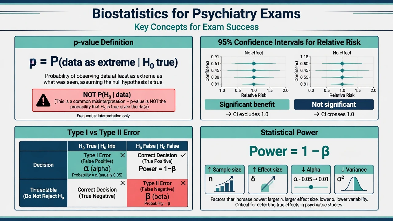
A p-value is the probability, under a specified statistical model that includes the null hypothesis (H0), of obtaining data as extreme as, or more extreme than, those observed.[2][3]
It is not: the probability that H0 is true given the data (that is a posterior; Bayes needed); the probability that results are due to chance in a colloquial sense; a measure of effect size or clinical importance; or a fixed reproducible property of the scientific claim across replications without further assumptions.[2][3]
Conventionally, alpha (α) = 0.05 means we pre-specify a Type I error rate of 5% for rejecting a true H0. Crossing p less than 0.05 is not a biological law — it is a long-run error-control convention that collapses under selective reporting and multiple testing.[2][18]
Confidence intervals — precision you can defend
A 95% confidence interval is constructed so that, under repeated sampling and correct model assumptions, 95% of such intervals would contain the true parameter. For a single study, interpret the interval as a range of values reasonably compatible with the data under the model — not as a probability that the true value lies inside this interval in a Bayesian sense without priors.[1][2]
Exam reading rules for ratios (RR, OR, HR): if the 95% CI includes 1, the conventional null of no relative association is not rejected at α = 0.05 for the corresponding test; if the CI lies entirely below 1, data support reduced event rate (for a bad outcome) or reduced hazard; if entirely above 1, data support increased rate/hazard. Width is clinical: a RR of 0.80 (0.20–3.20) is essentially uninformative; a RR of 0.80 (0.72–0.89) is precise.[1][2]
For risk differences, the null is 0 (not 1). Always know which scale you are on.[1]
Type I error, Type II error, and power
| H0 true (no real effect) | H0 false (real effect) | |
|---|---|---|
| Reject H0 | Type I error (false positive), rate α | Correct detection (true positive) |
| Do not reject H0 | Correct retention | Type II error (false negative), rate β |
Type I error is a false positive rejection of a true null; Type II error is a false negative failure to reject a false null — the complementary rates α and β frame long-run error control for hypothesis tests.[5][2]
Power = 1 − β = probability of detecting a specified true effect (rejecting H0 when a given alternative is true). Power rises with larger sample size, larger true effect, higher α, and lower outcome variance; it falls with multiple testing penalties, measurement error, and non-adherence that dilutes effects.[5][6]
Classic surveys showed many "negative" trials were too small to exclude clinically important benefits — underpowered negatives are inconclusive, not proof of no effect.[4][5] Sample-size calculation should be pre-specified with primary outcome, minimal important difference, α, power, and expected control rate; post-hoc power after seeing a non-significant result is largely uninformative once the CI is available.[6]
Absolute and relative treatment effects
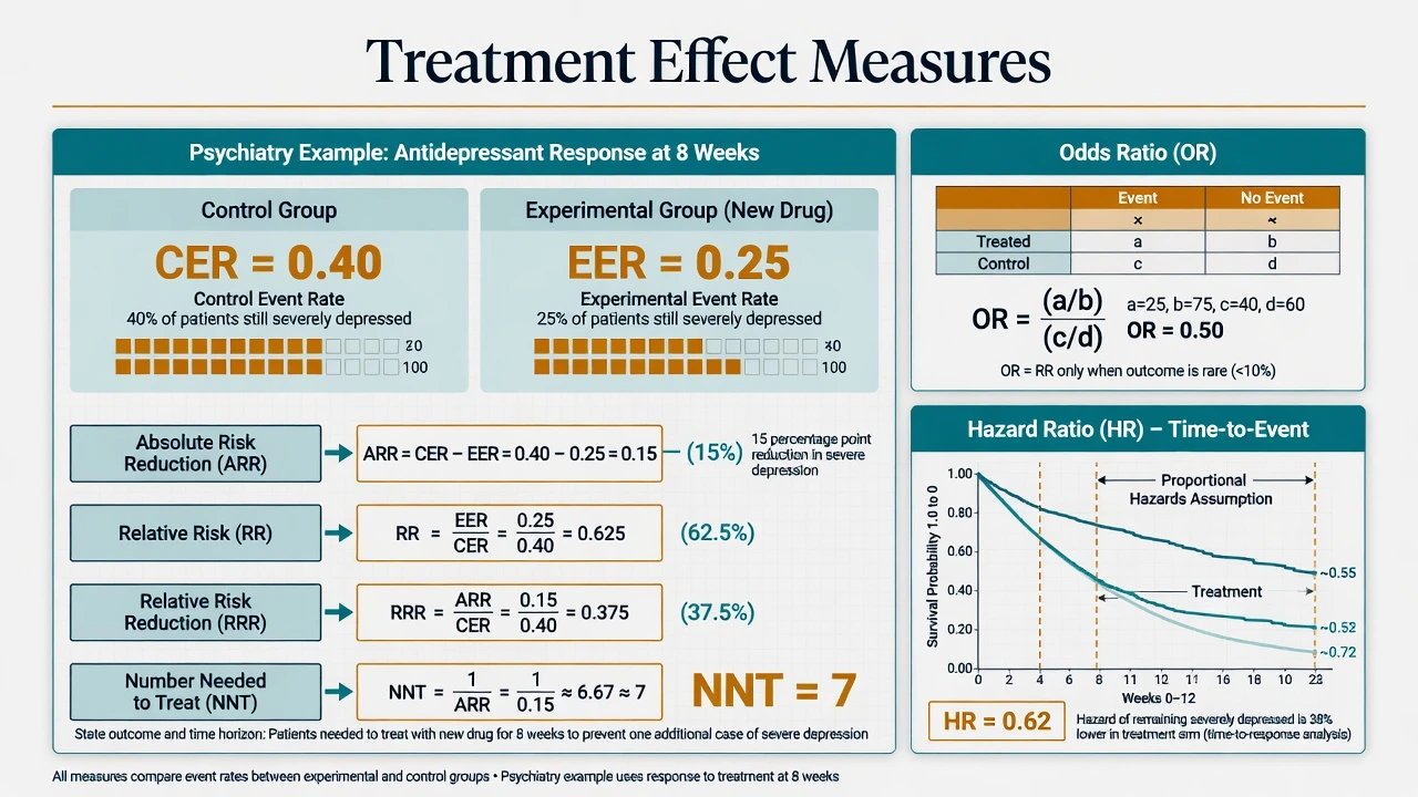
Define event rates for a dichotomous outcome over a stated time: CER = control event rate; EER = experimental event rate.[7][8]
Then (for a bad outcome you want fewer of): ARR (absolute risk reduction) = CER − EER; RR (relative risk / risk ratio) = EER / CER; RRR (relative risk reduction) = (CER − EER) / CER = 1 − RR; NNT = 1 / ARR (round carefully; always state outcome and duration); NNH uses absolute risk increase for harms.[7][8]
For a good outcome (e.g. response), the absolute benefit is EER − CER and NNT = 1 / absolute benefit.[7][8]
Worked psychiatry-style example (response at 8 weeks): EER 50%, CER 35% → absolute benefit 15% (0.15) → NNT ≈ 7 for one extra responder over 8 weeks. RRR = 0.15/0.35 ≈ 43% — the number that looks impressive in abstracts without absolute rates.[8]
Odds ratio vs relative risk
Odds = probability / (1 − probability). OR compares odds between groups. Logistic regression and case-control designs naturally yield ORs. When the outcome is uncommon (rule-of-thumb often less than about 10%), OR ≈ RR. When the outcome is common, OR is farther from 1 than RR and will overstate relative risk if misread as RR.[9][10]
Hazard ratio
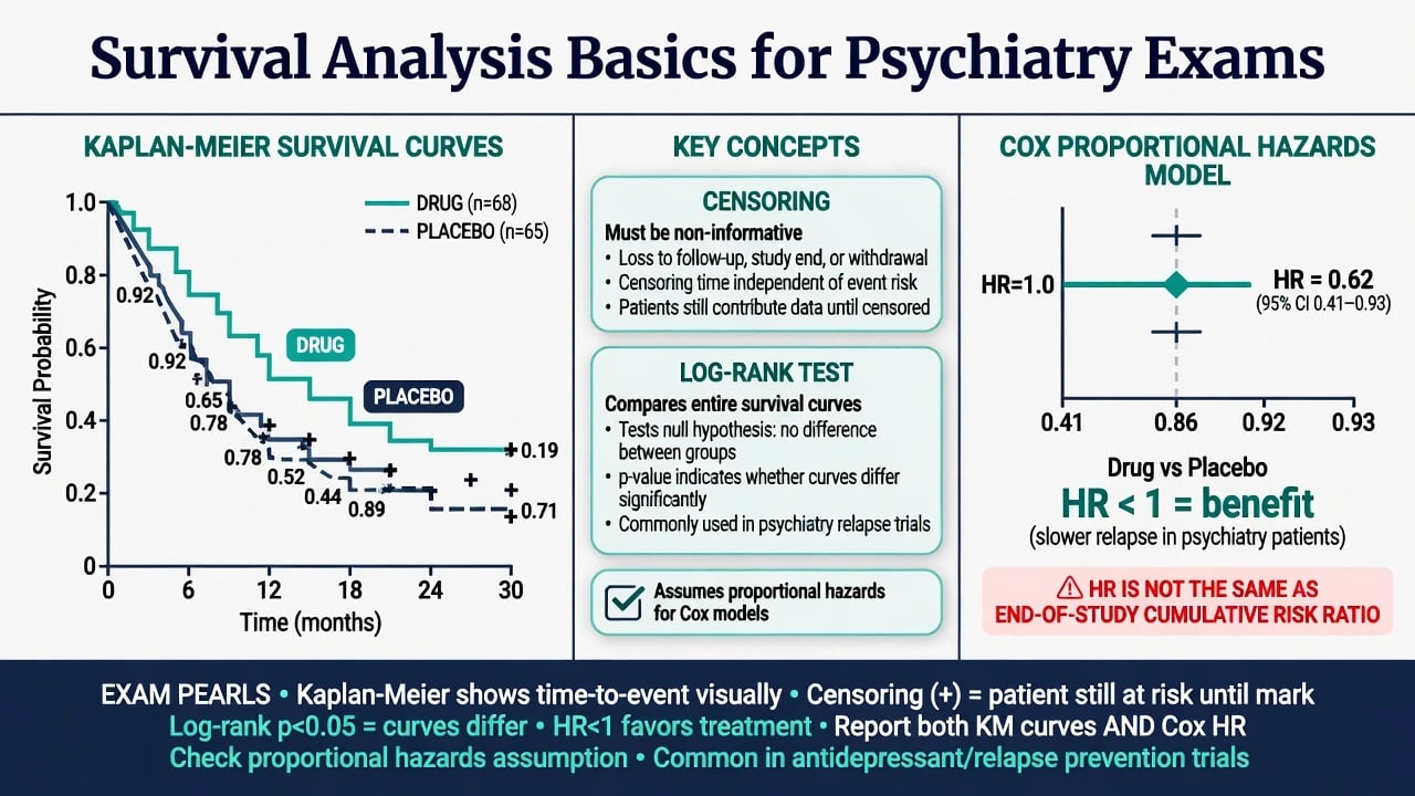
The hazard is an instantaneous event rate among those still at risk. A hazard ratio (HR) from a Cox model compares hazards between groups under a proportional hazards assumption (HR roughly constant over time). HR less than 1 for time-to-relapse means slower instantaneous relapse rate on treatment — it is not identical to the cumulative risk ratio at the end of follow-up.[11]
Relative risk (RR)
- Ratio of cumulative risks over a fixed period
- Intuitive for RCTs with complete follow-up
- Null = 1; pair with ARR/NNT
Odds ratio (OR)
- Ratio of odds; natural for logistic and case-control
- Approximates RR when events rare
- Misread as RR when events common → exaggeration
Hazard ratio (HR)
- Ratio of instantaneous hazards over time
- From survival models (Cox)
- Not interchangeable with end-of-study RR without care
Diagnostic accuracy — Sn, Sp, predictive values, LRs, ROC
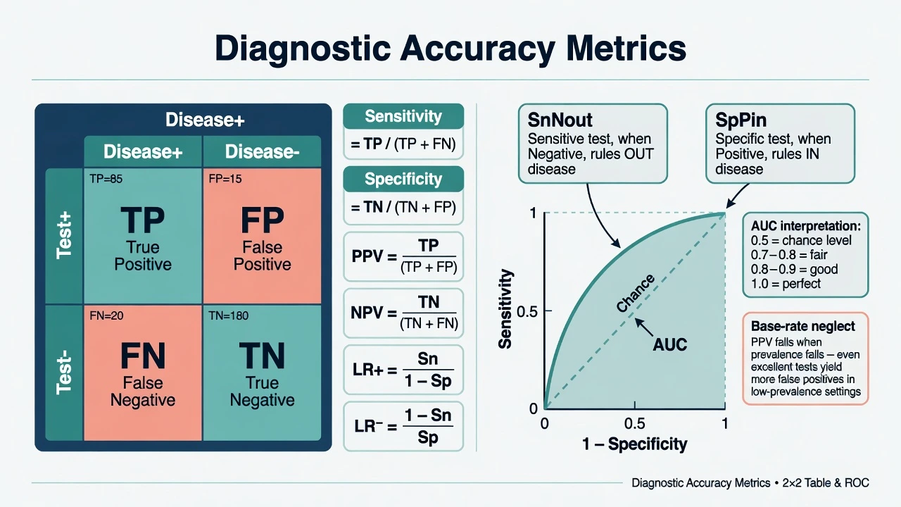
Build a 2 × 2 against a reference standard (Test+/− by Disease+/− yielding TP, FP, FN, TN). Sensitivity (Sn) = TP / (TP + FN); Specificity (Sp) = TN / (TN + FP); PPV = TP / (TP + FP); NPV = TN / (TN + FN).[12][13]
Sn and Sp are properties of the test in a spectrum of patients; PPV and NPV also depend on prevalence (pre-test probability).[12][13][20]
Mnemonics: SnNout — highly Sensitive test, Negative result helps rule out. SpPin — highly Specific test, Positive result helps rule in.[12][20]
Likelihood ratios (prevalence-independent expressions of test strength): LR+ = Sn / (1 − Sp); LR− = (1 − Sn) / Sp. Rough teaching thresholds: LR+ greater than about 10 often provides strong evidence to rule in; LR− less than about 0.1 often strong evidence to rule out — context still matters.[15][20]
ROC and AUC
A receiver operating characteristic (ROC) curve plots sensitivity against (1 − specificity) as the diagnostic threshold moves. The area under the curve (AUC) equals the probability that a randomly chosen diseased subject ranks higher on the test than a randomly chosen non-diseased subject. AUC 0.5 = chance; 1.0 = perfect separation.[14][16] Choosing a cut-point trades false negatives against false positives; exam stems often ask you to reason about screening (favour Sn) versus confirmation (favour Sp).
STARD-aligned reporting expects complete 2 × 2 counts, spectrum description, and blind comparison to a reference standard — not marketing-grade "accuracy 95%" slogans.[21]
Survival analysis basics
Time-to-event data include patients who never experience the event during observation (censored). The Kaplan–Meier estimator produces a stepped survival curve; patients contribute until event or censoring. Valid interpretation assumes non-informative censoring (censoring unrelated to prognosis beyond covariates handled by the design/model).[17]
The log-rank test compares survival curves between groups under a null of no difference in survival distributions. Multivariable adjustment and HR estimation typically use Cox proportional hazards models, requiring roughly proportional hazards over time (checkable with log-minus-log plots or time interactions at deeper levels).[11][17]
Psychiatry uses: time to relapse after antipsychotic discontinuation, time to hospitalisation, time to suicide attempt (sparse events → wide CIs), and maintenance antidepressant trials — all of which need survival methods rather than naive end-of-study proportions alone.[11][17]
Multiplicity, false findings, and meta-analytic awareness
When many endpoints, subgroups, and interim looks are mined without correction, family-wise Type I error explodes. Small effects, flexible analyses, and publication bias make many published "significant" findings unreliable as claimed.[18] For pooled estimates, I-squared describes the percentage of variability across studies attributable to heterogeneity rather than chance; high I-squared demands clinical interrogation before trusting a single diamond.[22] GRADE rates certainty down for imprecision (wide CIs, few events) among other domains — biostatistical literacy feeds guideline language.[19]
Exam calculation algorithm (60-second drill)
Identify the metric asked; write the formula; confirm numerator and denominator (good vs bad event; diseased vs tested); compute carefully; state outcome definition, time horizon, and population; refuse RRR-only marketing if absolute rates are missing.[1][8][12]
Calculation discipline under pressure
PAPERS
NNT, RR, OR, Sn, Sp, PPV, LR, HR — name it
Write CER/EER or 2×2 before algebra
Correct arm in numerator; risk difference vs ratio null
NNT with time and outcome; CI not just p
No RRR without ARR; no p as P(H0)
Wide CI or underpowered negative = inconclusive
These steps operationalise estimation-first teaching and protect against relative-risk spin and p-value mysticism under exam pressure.[1][2][8]
Regional and board notes
FRANZCP embeds biostats inside EBM/viva critique: expect NNT language, CI reading, and refusal of underpowered equivalence claims alongside clinical applicability. RANZCP guidance increasingly uses GRADE-style certainty language; imprecision is a core downgrade domain when CIs are wide or events few.[19]
MD/DNB and NEET-SS theory/viva expect formulae, worked 2×2 tables, and survival vocabulary with psychiatry trial examples. Across boards, imprecision (wide CIs, few events) should temper practice change language.[19]
Special populations — transfer of numbers
Child and adolescent trials often have small N → low power and wide CIs. Older adult trials exclude frailty and polypharmacy → baseline risk (and thus NNT) may not transfer. Perinatal safety signals are often observational ORs with rare outcomes — wide CIs and confounding dominate. Intellectual disability populations may have noisier continuous measures (measurement error raises variance and lowers power). Cultural or language mismatch can degrade scale validity and shift MCID interpretation. Always ask whether the absolute baseline risk in this patient matches the trial CER before importing an NNT.[5][6][8][10]
Complications and classic traps
Classic traps include equating p less than 0.05 with clinical importance; quoting RRR without ARR/NNT; reading OR as RR when response rates are common; calling a CI that includes 1 a "positive trend"; claiming equivalence from underpowered negatives; confusing Sn with PPV; omitting the NNT time frame; treating HR as the end-of-study cumulative RR; and ignoring informative censoring when dropouts differ by severity.[2][4][8][9][11][13]
Prognosis for practice change
Change practice when internal validity is acceptable, absolute benefit is meaningful for this baseline risk, the CI excludes trivial effects on patient-important outcomes, and harms, values, and resources are integrated. A statistically significant but tiny ARR with NNT in the hundreds for a soft continuous surrogate rarely justifies wholesale protocol change — GRADE imprecision language is useful here.[1][8][19]
Exam pearls (memorise)
NNT = 1 / |absolute benefit| with outcome and duration; p = P(data as extreme or more | H0 and model), not P(H0|data); a 95% CI for RR/OR/HR including 1 means non-significance at conventional α; OR ≈ RR only when the outcome is rare; use SnNout / SpPin and LRs to move pre-test to post-test odds; PPV falls as prevalence falls; absence of evidence ≠ evidence of absence; plan power before the study and read the CI afterward; HR ≠ end-of-study RR; continuous primaries do not yield NNT without dichotomisation.[1][2][4][8][9][11][12][13][15]
Related topics
Pair this page with critical appraisal (bias, RoB 2, CONSORT/PRISMA), research methods (design taxonomy), and clinical topics that supply real effect sizes (antidepressants, antipsychotics, suicide risk).[3][18][19]
References
- [1]Gardner MJ, Altman DG Confidence intervals rather than P values: estimation rather than hypothesis testing Br Med J (Clin Res Ed), 1986.PMID 3082422
- [2]Greenland S, Senn SJ, Rothman KJ, et al. Statistical tests, P values, confidence intervals, and power: a guide to misinterpretations Eur J Epidemiol, 2016.PMID 27209009
- [3]Sterne JA, Davey Smith G Sifting the evidence—what's wrong with significance tests? BMJ, 2001.PMID 11159626
- [4]Altman DG, Bland JM Absence of evidence is not evidence of absence BMJ, 1995.PMID 7647644
- [5]Freiman JA, Chalmers TC, Smith H Jr, Kuebler RR The importance of beta, the type II error and sample size in the design and interpretation of the randomized control trial. Survey of 71 "negative" trials N Engl J Med, 1978.PMID 355881
- [6]Schulz KF, Grimes DA Sample size calculations in randomised trials: mandatory and mystical Lancet, 2005.PMID 15823387
- [7]Laupacis A, Sackett DL, Roberts RS An assessment of clinically useful measures of the consequences of treatment N Engl J Med, 1988.PMID 3374545
- [8]Cook RJ, Sackett DL The number needed to treat: a clinically useful measure of treatment effect BMJ, 1995.PMID 7873954
- [9]Bland JM, Altman DG Statistics notes. The odds ratio BMJ, 2000.PMID 10827061
- [10]Grimes DA, Schulz KF Making sense of odds and odds ratios Obstet Gynecol, 2008.PMID 18238982
- [11]Spruance SL, Reid JE, Grace M, Samore M Hazard ratio in clinical trials Antimicrob Agents Chemother, 2004.PMID 15273082
- [12]Altman DG, Bland JM Diagnostic tests. 1: Sensitivity and specificity BMJ, 1994.PMID 8019315
- [13]Altman DG, Bland JM Diagnostic tests 2: Predictive values BMJ, 1994.PMID 8038641
- [14]Altman DG, Bland JM Diagnostic tests 3: receiver operating characteristic plots BMJ, 1994.PMID 8044101
- [15]Deeks JJ, Altman DG Diagnostic tests 4: likelihood ratios BMJ, 2004.PMID 15258077
- [16]Hanley JA, McNeil BJ The meaning and use of the area under a receiver operating characteristic (ROC) curve Radiology, 1982.PMID 7063747
- [17]Bland JM, Altman DG Survival probabilities (the Kaplan-Meier method) BMJ, 1998.PMID 9836663
- [18]Ioannidis JPA Why most published research findings are false PLoS Med, 2005.PMID 16060722
- [19]Guyatt GH, Oxman AD, Vist GE, et al; GRADE Working Group GRADE: an emerging consensus on rating quality of evidence and strength of recommendations BMJ, 2008.PMID 18436948
- [20]Jaeschke R, Guyatt GH, Sackett DL Users' guides to the medical literature. III. How to use an article about a diagnostic test. B. What are the results and will they help me in caring for my patients? JAMA, 1994.PMID 8309035
- [21]Bossuyt PM, Reitsma JB, Bruns DE, et al; STARD Group STARD 2015: an updated list of essential items for reporting diagnostic accuracy studies BMJ, 2015.PMID 26511519
- [22]Higgins JP, Thompson SG, Deeks JJ, Altman DG Measuring inconsistency in meta-analyses BMJ, 2003.PMID 12958120