Psych · Foundations — epidemiologic methods for psychiatry
Epidemiologic methods for psychiatry
Also known as Psychiatric epidemiology methods · Incidence and prevalence · Person-time · Attributable risk · Population attributable fraction · Confounding · Effect modification · Survey sampling · Screening epidemiology · Causal inference · Standardisation of rates
Exam-exhaustive epidemiologic methods for FRANZCP and MRCPsych: frequency measures (incidence, prevalence, person-time), association and impact (RR, OR, RD, AR, PAF), bias/confounding/effect modification, survey design, screening metrics and Wilson–Jungner-style criteria, standardisation, and causal language (Hill, DAG awareness). Distinct from study-design taxonomy, pure biostat drills, and public-mental-health service planning.
On this page & tools
Your progress
Saved locally on this device.
10 MCQs with explanations
Target exams
Red flags
This page is the measurement and inference toolkit of psychiatric epidemiology. Research methods choose the design skeleton; biostatistics supplies estimation and error control arithmetic; public mental health applies burden and services. Examiners (FRANZCP written/viva, MRCPsych Paper A/B methods, ABPN EBM, MD/DNB theory) test whether you can name the right measure, defend the denominator, and refuse causal overclaim.[1][2][6]
Definition and classification
Epidemiology studies the distribution and determinants of health states in populations and applies that knowledge to control health problems. In psychiatry, that means counting cases under a case definition, estimating frequency, relating exposures to outcomes, and interpreting associations under bias and causal assumptions.[1][2]
| Layer | Question it answers | Not the same as |
|---|---|---|
| Frequency | How common / how often new? | Clinical severity of one patient |
| Association | Is exposure related to outcome? | Proof of mechanism |
| Impact | How much disease might be attributed / prevented if causal? | Automatically actionable without ethics and feasibility |
| Inference | How strong is the causal claim? | STROBE compliance alone |
Frequency answers how common or how often new cases arise; association answers whether exposure and outcome co-vary; impact and causal inference demand additional assumptions beyond a single crude association.[1][5][8]
Frequency measures — definitions examiners expect
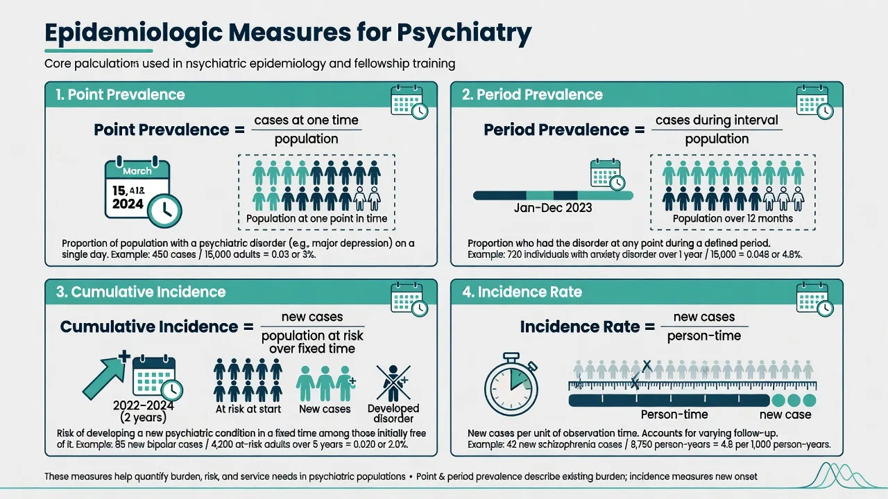
Point prevalence = number of existing cases at a specified time / population at that time. Period prevalence = number of people who were cases at any time during an interval (for example 12 months) / population. Lifetime prevalence = ever meeting criteria up to assessment — useful for cumulative burden and age-of-onset work, poor for current service need because of recall and recovery.[14][15]
Cumulative incidence (risk) = new cases during a fixed period / population initially at risk (closed cohort ideal). Incidence rate (incidence density) = new cases / person-time at risk — preferred when people enter and leave follow-up unequally.[3]
Steady-state teaching rule: prevalence ≈ incidence × average duration of the disease state (when population is stable and migration/competing risks are ignored at exam level). Chronic, long-duration disorders (schizophrenia, some personality pathology) can have moderate incidence yet high prevalence; brief remitting states reverse the pattern.[1][3]
Crude, specific, and standardised rates
A crude rate uses the whole population denominator. Specific rates stratify (age-, sex-, diagnosis-specific). Standardisation reweights rates to a common age structure so two regions or eras can be compared without pure demographic confounding by age mix. Direct standardisation applies stratum-specific rates to a standard population; indirect standardisation (SMR-style thinking) compares observed to expected events. Standardisation does not fix unmeasured confounding of exposure–disease relationships inside analytic studies.[1][2]
Measures of association and impact
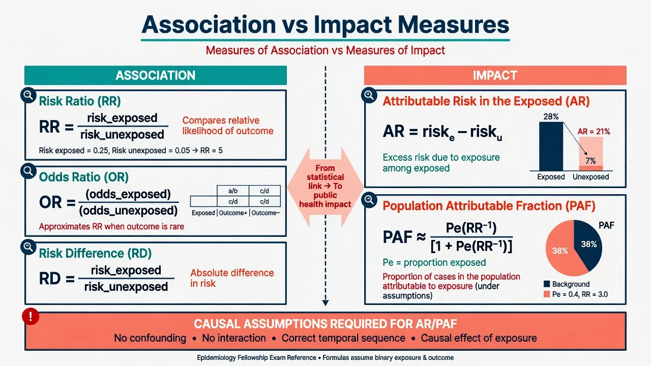
For a binary outcome over a stated risk period among exposed (E) and unexposed (U): Risk ratio (relative risk, RR) = risk_E / risk_U; Risk difference (RD) = risk_E − risk_U; Odds ratio (OR) = odds_E / odds_U (natural for logistic models and many case-control analyses).[1][3][4]
When the outcome is uncommon, OR ≈ RR. When the outcome is common, OR moves farther from 1 than RR — reading OR as RR exaggerates association strength.[4]
Attributable risk in the exposed (AR) = risk_E − risk_U (same algebra as RD for a harmful exposure) — the excess risk among exposed if the association is causal. Attributable fraction among the exposed = (RR − 1) / RR under standard assumptions. Population attributable fraction (PAF) estimates the proportion of cases in the whole population that would not occur if the exposure were eliminated and the association were causal and unbiased; a common teaching formula when RR and exposure prevalence (Pe) are available is PAF = Pe(RR − 1) / [1 + Pe(RR − 1)]. PAF is highly assumption-dependent and is misused when exposures are correlated, misclassified, or non-causal.[8]
RR / OR
- Relative association
- Null = 1
- OR ≈ RR only if outcome rare
Risk difference
- Absolute association
- Null = 0
- Closest to clinical/public-health scale
AR / PAF
- Impact if causal
- Needs unbiased RR and exposure prevalence
- Do not naively sum correlated PAFs to 100%+
Bias, confounding, and effect modification
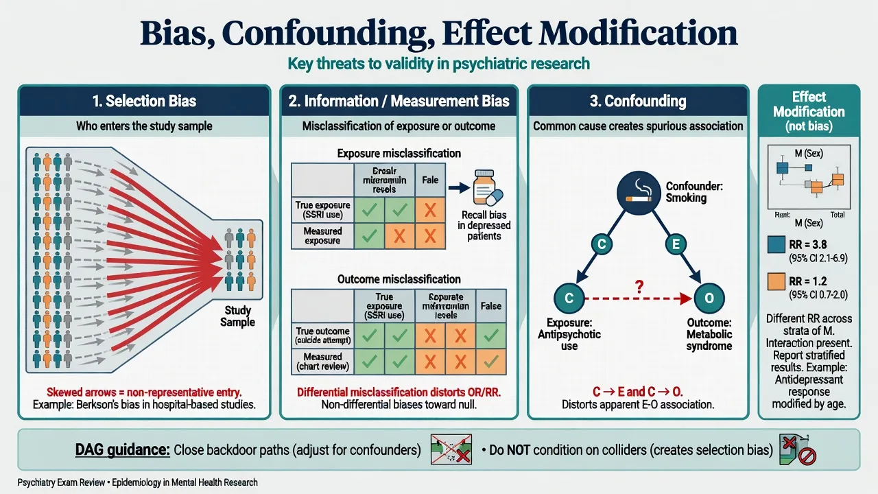
Three classic families distort observational associations: selection bias (who enters or remains in the sample), information/measurement bias (misclassification of exposure, outcome, or covariates), and confounding (a common cause of exposure and outcome mixing effects).[2][7]
Confounding is structural: C causes E and C causes O (or a proxy path), so the crude E–O association is partly C’s effect. Control is by design (restriction, matching, randomisation in trials) or analysis (stratification, multivariable models) after measuring sufficient confounders. Effect modification (interaction) means the effect of E on O differs across levels of M — the scientifically correct move is often to report stratum-specific estimates, not to force a single adjusted summary that hides heterogeneity.[2][9]
Directed acyclic graphs (DAGs) make this exam-useful: identify backdoor paths from E to O that must be blocked for an unconfounded estimate; avoid conditioning on colliders (common effects), which can open bias paths.[9]
Psychiatry-specific threats: recall bias in case-control trauma studies; prevalence–incidence (Neyman) bias when late sampling of chronic survivors misses fatal or remitted early cases; confounding by indication in pharmacoepidemiology; protopathic bias when prodromal illness changes exposure (for example self-medication before diagnosis); non-response when stigma or severity drives refusal in household surveys.[2][4][7][15]
Association versus causation
An association is a statistical relation. Causation is a counterfactual claim: intervening on exposure would change outcome risk. Hill’s classic viewpoints (strength, consistency, specificity, temporality, biological gradient, plausibility, coherence, experiment, analogy) are weight-of-evidence aids, not a pass/fail checklist; temporality is logically required for cause preceding effect.[5] Randomised experiments strengthen causal inference when ethical and feasible; many psychiatric harm questions (prenatal exposures, childhood maltreatment) remain observational and demand triangulation, bias analysis, and humility.[2][5]
Survey methods and case definition
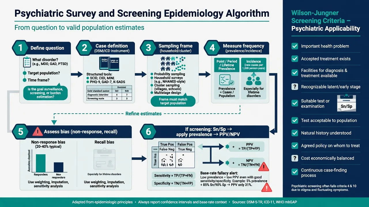
Community psychiatric epidemiology rests on: (1) a target population and sampling frame; (2) a probability sampling plan (simple, stratified, cluster, multi-stage); (3) a case definition operationalised with structured interviews or validated instruments; (4) a recall window (2-week, 12-month, lifetime); (5) response rate and non-response analysis; (6) weighting for design and non-response.[14][15][6]
Landmark survey programmes (for example NCS-R, WHO World Mental Health surveys) illustrate that method choices change prevalence: instrument version, hierarchy rules, severity thresholds, and cultural adaptation all move estimates.[14][15] Clinical samples answer different questions — treated prevalence, severity mix, dual diagnosis — and must not be generalised as community rates.
Ecological studies relate area-level exposures to area-level rates. They can generate hypotheses and evaluate population policies but invite the ecological fallacy if group associations are read as individual-level effects without multi-level design.[1][2]
STROBE provides a reporting skeleton for observational work (objectives, setting, participants, variables, bias, study size, statistical methods, participants flow, descriptive data, outcome data, main results, limitations) — transparency, not a quality medal.[6]
Screening epidemiology
Screening applies a test to asymptomatic or unselected people to identify probable cases for further assessment. Sensitivity and specificity characterise test performance against a reference standard; PPV and NPV also depend on prevalence (pre-test probability).[10][11]
Classic trap: a depression or psychosis risk screen with impressive Sn/Sp in a high-prevalence clinic yields a low PPV in a low-prevalence community or school sample — most positives are false positives, with stigma and resource costs.[11] STARD-aligned reporting expects full 2×2 counts, spectrum description, and blind comparison to a reference standard.[16]
Wilson and Jungner’s classic screening criteria (important condition, accepted treatment, facilities, latent stage, suitable test, acceptable test, understood natural history, agreed policy, cost balance, continuing process) remain a scaffold; modern updates emphasise equity, programme quality, and informed choice — not gadget novelty alone.[12] Rose’s insight still frames prevention epidemiology: shifting the population distribution of risk often prevents more cases than only treating the high-risk tail (with the prevention paradox).[13]
Worked psychiatry-style calculations (exam drill)
A. Period prevalence. Of 2,000 adults surveyed, 240 met 12-month criteria for any mood or anxiety disorder → period prevalence = 240/2000 = 0.12 (12%). State instrument and window.[15]
B. Incidence rate. Inception cohort of 500 people at risk; 20 develop first-episode psychosis over 2,000 person-years → incidence rate = 20/2000 = 0.01 per person-year (10 per 1,000 person-years).[3]
C. RR and AR. Risk of major depression over 1 year: exposed to severe childhood adversity 0.20; unexposed 0.08 → RR = 0.20/0.08 = 2.5; AR = 0.12. If Pe in the population is 0.25 and assumptions hold, PAF = 0.25×1.5 / [1 + 0.25×1.5] = 0.375/1.375 ≈ 0.27 (27%) — report as model-based, not destiny.[8]
D. Screening PPV intuition. Sn 0.90, Sp 0.90, prevalence 0.02 in 10,000 people → about 180 true positives and 882 false positives among screen-positives → PPV ≈ 180/(180+882) ≈ 17%. Same test at prevalence 0.20 yields much higher PPV.[10][11]
Epidemiology methods under pressure
RATES
Incidence vs prevalence vs RR vs PAF — name it
People, person-time, or cases only?
Point, 12-month, lifetime, cohort years
Selection, information, confounding, modification
Association ≠ causation; PAF needs assumptions
These steps keep frequency, association, bias naming, and causal humility aligned under exam time pressure.[1][2][5][8]
Acute exam move when a claim is invalid
Identify the fatal flaw in one sentence (wrong measure, wrong denominator, unadjusted confounding, base-rate neglect, reverse causation), restate what can be claimed, and name the design or analysis that would strengthen inference (longitudinal person-time, better sampling, STROBE-complete reporting, randomised prevention trial when ethical).[2][6][7]
Subtypes and classic scenarios
| Scenario | Preferred frequency / design logic | Main threat |
|---|---|---|
| Catchment 12-month burden | Probability survey, period prevalence | Non-response, instrument choice |
| First-episode psychosis onset | Inception cohort, incidence rate | Incomplete case finding |
| Clozapine agranulocytosis risk factors | Case-control or nested case-control | Control selection, confounding |
| Suicide after discharge | Cohort with person-time; competing risks awareness | Loss to follow-up, rare events |
| Area deprivation and admission rates | Ecological / multi-level | Ecological fallacy, bed supply |
| School mental-health screen | Screening metrics at low prevalence | False-positive burden |
| Suicide cluster | Temporal-spatial excess vs chance | Media contagion, small-number noise |
Nested case-control studies sample cases and controls from within a defined cohort, preserving a study base and enabling efficient biomarker or costly exposure measurement while retaining person-time logic of the parent cohort.[3][4]
Special populations
Children and adolescents: multi-informant case definition (child, parent, teacher), developmental diagnostic thresholds, and cluster sampling by school (design effect).[1] Older adults: competing mortality, dementia ascertainment challenges, survivor bias if only community-dwelling elders are sampled. Perinatal: short, sharp risk windows; pregnancy cohorts with gestational timing of exposure. Intellectual disability: adaptive diagnostic methods beyond standard CIDI-style interviews; sampling frames miss institutionalised or informal carers. Indigenous and culturally diverse populations: community governance, cultural safety of instruments, mobile or non-household populations outside standard frames.[15] Forensic and inpatient samples: extreme selection — high comorbidity and severity; never quote as community prevalence.
Regional and board notes
FRANZCP embeds epidemiologic literacy in EBM critique and public-health MEQs: expect clean definitions of incidence/prevalence, bias naming, and cautious PAF language when discussing prevention and Closing the Gap–adjacent social determinants. RANZCP-facing service arguments still need population denominators, not ward census anecdotes.[6][15]
MD/DNB and NEET-SS viva favour crisp formulae, bias names, Hill criteria, and worked prevalence/incidence stems with psychiatry examples.[1][5]
Complications and classic traps
Traps include using lifetime prevalence for current bed planning; equating admission rates with community incidence; calling a single clinic series a prevalence study without a population denominator; reading OR as RR when depression “response” or “caseness” is common; adjusting for mediators (for example current substance use on the path from trauma to psychosis) and declaring no effect; conditioning on colliders; ignoring design effects of cluster sampling; and marketing community screens without PPV at the true base rate.[2][4][7][8][9][11]
Prognosis for claims and policy
Frequency estimates prioritise problems; association and impact estimates, if causal and unbiased, prioritise prevention targets; only intervention evidence (or exceptionally strong causal inference for harmful exposures) should rewrite treatment protocols. Rose’s population strategy and high-risk strategies are complementary, not mutually exclusive — method choice follows the prevention question.[8][13][5]
Exam pearls (memorise)
Prevalence ≈ incidence × duration (teaching steady state); incidence needs new cases + time; person-time for unequal follow-up; period (for example 12-month) prevalence usually beats lifetime for current need; OR ≈ RR only if outcome rare; confounding ≠ effect modification; PAF needs causal assumptions (Rockhill); PPV falls as prevalence falls; association ≠ causation — Hill is weight of evidence with temporality essential; STROBE is reporting transparency, not proof of validity; clinical samples ≠ community rates; name selection, information, confounding before arguing policy.[1][2][3][5][6][8][11]
Related topics
Pair with research methods (design taxonomy), biostatistics (CI, NNT, power), advanced critical appraisal (RoB tools, GRADE), public mental health (GBD, treatment gap, prevention packages), and measurement-based care (scale psychometrics as information bias control).[1][6][16]
References
- [1]Grimes DA, Schulz KF An overview of clinical research: the lay of the land Lancet, 2002.PMID 11809203
- [2]Grimes DA, Schulz KF Bias and causal associations in observational research Lancet, 2002.PMID 11812579
- [3]Grimes DA, Schulz KF Cohort studies: marching towards outcomes Lancet, 2002.PMID 11830217
- [4]Grimes DA, Schulz KF Case-control studies: research in reverse Lancet, 2002.PMID 11844534
- [5]Hill AB The environment and disease: association or causation? Proc R Soc Med, 1965.PMID 14283879
- [6]von Elm E, Altman DG, Egger M, Pocock SJ, Gøtzsche PC, Vandenbroucke JP; STROBE Initiative The Strengthening the Reporting of Observational Studies in Epidemiology (STROBE) statement: guidelines for reporting observational studies Lancet, 2007.PMID 18064739
- [7]Sackett DL Bias in analytic research J Chronic Dis, 1979.PMID 447779
- [8]Rockhill B, Newman B, Weinberg C Use and misuse of population attributable fractions Am J Public Health, 1998.PMID 9584027
- [9]Greenland S, Pearl J, Robins JM Causal diagrams for epidemiologic research Epidemiology, 1999.PMID 9888278
- [10]Altman DG, Bland JM Diagnostic tests. 1: Sensitivity and specificity BMJ, 1994.PMID 8019315
- [11]Altman DG, Bland JM Diagnostic tests 2: Predictive values BMJ, 1994.PMID 8038641
- [12]Andermann A, Blancquaert I, Beauchamp S, Déry V Revisiting Wilson and Jungner in the genomic age: a review of screening criteria over the past 40 years Bull World Health Organ, 2008.PMID 18438522
- [13]Rose G Sick individuals and sick populations Int J Epidemiol, 2001.PMID 11416056
- [14]Kessler RC, Berglund P, Demler O, Jin R, Merikangas KR, Walters EE Lifetime prevalence and age-of-onset distributions of DSM-IV disorders in the National Comorbidity Survey Replication Arch Gen Psychiatry, 2005.PMID 15939837
- [15]Demyttenaere K, Bruffaerts R, Posada-Villa J, et al. Prevalence, severity, and unmet need for treatment of mental disorders in the World Health Organization World Mental Health Surveys JAMA, 2004.PMID 15173149
- [16]Bossuyt PM, Reitsma JB, Bruns DE, et al; STARD Group STARD 2015: an updated list of essential items for reporting diagnostic accuracy studies BMJ, 2015.PMID 26511519